Notes
Article history
The research reported in this issue of the journal was funded by the HS&DR programme or one of its proceeding programmes as project number 09/2000/47. The contractual start date was in April 2011. The final report began editorial review in October 2012 and was accepted for publication in March 2013. The authors have been wholly responsible for all data collection, analysis and interpretation, and for writing up their work. The HS&DR editors and production house have tried to ensure the accuracy of the authors’ report and would like to thank the reviewers for their constructive comments on the final report document. However, they do not accept liability for damages or losses arising from material published in this report.
Declared competing interests of authors
Nancy Devlin has chaired the EuroQoL Group, and the Office of Health Economics has received payments of various kinds for her work in the area of health outcome measures. The other authors declare no competing interests.
Permissions
Copyright statement
© Queen’s Printer and Controller of HMSO 2014. This work was produced by Street et al. under the terms of a commissioning contract issued by the Secretary of State for Health. This issue may be freely reproduced for the purposes of private research and study and extracts (or indeed, the full report) may be included in professional journals provided that suitable acknowledgement is made and the reproduction is not associated with any form of advertising. Applications for commercial reproduction should be addressed to: NIHR Journals Library, National Institute for Health Research, Evaluation, Trials and Studies Coordinating Centre, Alpha House, University of Southampton Science Park, Southampton SO16 7NS, UK.
Chapter 1 Introduction
Patient-reported outcome measures (PROMs) are instruments that capture the patient’s own assessment of his or her health. 1 By comparing these measures of health through time – for example, before and after treatment – changes in health can be identified and used to better understand the effect of health care. PROMs are already widely used for making some health-care decisions – for example, the National Institute for Health and Care Excellence (NICE) uses PROMs data to help establish the cost-effectiveness of health-care technologies. However, relatively little is known about the clinical effectiveness and cost-effectiveness of many services provided by the NHS in England in terms of their impact on patient-reported health.
Since April 2009, all providers of publicly funded inpatient care in the English NHS have been required to collect both generic and condition-specific instruments for four elective procedures: unilateral hip replacement, unilateral knee replacement, varicose vein surgery and groin hernia repairs. 2 Patients having these procedures are invited to report their health status before surgery, as well as 3 or 6 months after surgery.
The PROMs programme is unique internationally: the English NHS is the first health-care system in the world to require the routine collection of data on patient-reported health and the intention is to use these data to inform a wide range of NHS decisions. Clinical teams may use these data to monitor their own performance and to identify opportunities for improving the quality of services. Patients and their general practitioners may use the information to choose which hospital to attend for treatment. Commissioners of health-care services may use these data to establish which services, for which subgroups of patients, are most effective and best value for money.
One of the most important catalysts for the introduction of the PROMs programme was the aim of using these data to compare hospital performance. The changes in patients’ health status can be analysed to identify systematic variation across hospital providers and are expected to ‘provide an indication of the outcomes or quality of care delivered to NHS patients’. 2 The identification of which hospitals are most successful in improving patient health makes it possible to link rewards to that performance either indirectly, by patients choosing high-performing hospitals over poor performers, or directly by linking performance-related payments to achievements in terms of PROMs. Both are seen as having the potential to sharpen hospital incentives to improve quality. However, there are clearly risks associated with the use of PROMs in this context. First, different instruments for measuring patient-reported outcomes (PROs) are available. Results may be sensitive to the choice of instrument and patients may differ in what weight they attach to the different dimensions used to describe health status. Second, variations in PROMs performance across hospitals may relate to variations in resource use and costs. A better understanding of the inter-relationship between costs and health outcomes is even more important in times of economic constraint, when there is greater pressure to ensure that NHS resources are used to their full extent. If this inter-relationship is poorly understood, there is a danger that efforts to reduce costs may have an adverse effect on patient outcomes.
The overall aims of this project are to develop means to understand variation in outcomes and costs across hospitals in the English NHS. More specifically, we aim to (1) characterise variation in outcomes in ways that are intuitive to patients and consistent with the original format of the questionnaire, thereby helping them select a preferred provider of care and (2) assess the relationship between the cost and outcomes of the four elective procedures for which PROM data are collected and to determine the extent to which variations in outcome and cost ratios are due to differences in hospital performance. In meeting these aims we consider:
-
which PROMs instrument should be used to measure outcomes
-
the extent to which variations in outcomes and cost of treatment are due to patient characteristics
-
the relationship between outcomes and cost of treatment
-
the influence of the hospital on outcomes and cost of treatment
-
how robust these estimates of hospital influences are to choices about how to conduct the analyses.
The research we have conducted led to two distinct pieces of work that address different aspects of these aims. The first part of the empirical analysis focuses on econometric techniques to analyse variation in different dimensions of patient self-reported health status, e.g. limitations in mobility or self-care, or the level of pain/discomfort or anxiety experienced. The results of this analysis highlight variability in the impact that hospital providers have on different dimensions of health, and we make suggestions on how best to communicate such variability to patients and other non-technical audiences. Because this analysis is directly aimed at developing methods for hospital comparison when the aim is to inform patient choice, we do not consider treatment costs or hospital production constraints in our analysis. The second part of the empirical analysis focuses on the performance of hospitals in terms of the inter-relationship between patient-reported outcomes and resource use. These results are more relevant for commissioners of services and hospital providers than for patients in the English NHS, where the costs of care are not linked to any out-of-pocket payments.
The report is structured as follows. In Chapter 2 we sketch a conceptual framework that outlines the influences on patient outcomes, notably patient characteristics and the hospital in which they are treated; how to characterise outcomes; and the inter-relationship between outcomes and resource use. In Chapter 3 we describe how we have linked data from various sources and how outcomes, resource use and patient characteristics are measured. Chapter 4 is split into two parts according to the two broad research questions and each part reports the econometric models, the sample and the results for each question. We conclude with a discussion of the main insights from the project and some suggestions for future refinements should richer data capturing of individual characteristics become available.
Chapter 2 Conceptual framework
An agency model of health-care provision
Health care describes the activity of improving patients’ health or changing its trajectory by means of medical, surgical or preventative intervention. The underlying process can be considered as a production function, where the patient’s initial pretreatment health status, H 0, is transformed into a post-treatment health status, H 1. The difference between pre- and post-treatment health status is termed the health outcome. An individual patient’s health outcome is a function (f) of several other factors, notably the characteristics of the patient, X, and the quality, Q, of the treatment carried out, so that:
For the elective procedures we study, treatment is provided in hospital. Hospitals combine ‘factors of production’, including staff, equipment and capital to produce treatment, the quality of which is partly determined by the specific amounts and combination of the input factors. However, quality may also be influenced by other constraining factors that impact on production, such as the size of the hospital, the number of procedures performed and whether or not doctors have to balance delivery of care with teaching commitments. Denoting the hospital’s effort to provide high-quality care as E h and exogenous production constraints as Z, quality can be expressed as:
and combining both equations, we obtain
Similarly, the cost function can be defined analogously as:
where C is the measure of resource use for the individual patient, H 0 is the patient’s initial health status, X is a vector of patient characteristics, E c is effort exerted by the hospital to contain resource use and Z denotes exogenous production constraints.
A hospital may not put as much effort into securing the level of quality that patients would like, nor into managing resource use as much as the regulator would like, partly because efforts on both objectives are costly;3 however, it is difficult to prove this because effort is inherently difficult to observe. A suggested solution has been to undertake comparative analysis of hospital performance. By comparing hospitals against each other, insight can be gained into the underlying production process, the constraints on this process and the effort exerted by different hospitals. 4,5 This requires the analyst to be able to draw a clear distinction between variations caused by factors such as differing patient case mix and other factors, notably effort.
Using outcome measures to evaluate quality of care
Information about patients’ health before and after treatment can be used to inform the choice of prospective patients and assess hospital performance with respect to the effort put into advancing quality. Clinical measures, such as blood pressure or joint movement, describe patient health in physiological terms but do not capture other relevant aspects, particularly quality of life. 6 Only the patients themselves can give a full account of their perceived health and, therefore, patients are increasingly recognised by regulatory bodies as the preferred source of information about the effectiveness of care. 7,8 To reduce the level of complexity and minimise cognitive burden, instruments to measure PRO often focus on a restricted number of health dimensions. A patient’s overall health status, H, can then be characterised as a function of these dimensions, H d , so that
where d = 1, . . . , D is the health dimension considered and h is an aggregation function to be defined. For simplicity, we drop the index for time here, but it should be clear that the argument applies to both pre- and post-treatment health status.
Means of aggregating health dimensions into an overall score are available for a wide range of different instruments. The NHS Information Centre has developed a quality performance assessment methodology that builds on aggregate health scores and is currently being applied to the PROM data. 9 For the EuroQol-5D questionnaire (EQ-5D; European Quality of Life-5 Dimensions), aggregation involves calculating weighted EQ-5D utility scores, where the weights reflect the preferences of the general population in England. 10,11 Post-treatment utility scores are then regressed on the pretreatment scores and case-mix controls to measure variation across hospitals in terms of the change in utilities that they achieve. The use of aggregate scores facilitates statistical analysis and allows for direct ranking of hospitals; however, this comes at a price. We identify four reasons why, for the purpose of informing patient choice and facilitating best practice dissemination through publishing performance data, analysing disaggregated outcome data may be preferable.
First, no aggregation function is neutral and observed variations in health outcomes may be driven by the choice of function, not genuine variation in performance. 12 In some circumstances, one may be willing to accept the value judgement implied or explicitly expressed by the aggregation function. For example, the convention of using the preferences of the general public to aggregate EQ-5D profiles has a clearly articulated rationale in the context of cost-effectiveness analysis and decisions concerning the allocation of taxpayer funding. 13 However, it should be understood that measuring and valuing health are two genuinely different activities. The use of aggregate outcome data to inform patient choice raises normative concerns because it imposes a common valuation of health dimensions. In fact, reporting relative hospital performance with respect to changes in the EQ-5D utility, for example, would be justified only if all (prospective) patients were to share the same relative values; however, patients may be heterogeneous with respect to their relative valuations of health dimension, or their relative valuations may differ from those of the general public. 14–15 If so, analysing variation on the level of health dimensions may be more appropriate as it allows patients to apply their own values when interpreting performance data.
Second, the use of performance data derived from the EQ-5D utility scores may be limited by patients’ difficulties in interpreting these quantities. In a recent qualitative study, Hildon et al. 16 interviewed patients and clinicians about their views on different metrics of hospital PROM performance. 16 The results suggest that ‘for patients [. . .], unlike measures of height or weight, PRO [. . .] scores are unfamiliar and their values have no immediate meaning. It’s therefore necessary to transform them into interpretable forms, or indeed into experiences rather than metrics, to make them useful’. Furthermore, patients ‘could not distinguish between the four [metrics], but liked a percentage or what was for them intuitive scaling’. 16 By analysing hospital performance in terms of disaggregated outcome data, inferences about performance can be made using the same metric in which these data have been collected.
Third, any form of aggregation causes loss of detail and information. 17 Once constructed, an aggregated measure cannot reveal information about the underlying components and the degree to which hospital providers affect each of them. Certain hospitals may perform well on one dimension but fall short on another. For example, the EQ-5D measures health-related quality of life in terms of limitations on the patient’s mobility and mental health (anxiety/depression) as well as other dimensions. A specific hospital may be good at improving the patient’s post-treatment mobility, but may fail to provide the necessary care to alleviate the patient’s concerns about his or her health status and the security of the hip implant. Detailed information on the performance on each dimension can help to identify the source of this problem and foster improvement through learning from other hospitals’ best practice. 17
Fourth, there are statistical concerns arising from the analysis of aggregate health status. For example, most instruments used to measure PRO impose ordinal scales onto the health dimension under consideration. The reported health status is the result of a censoring process in which patients classify their continuous, underlying health to a limited set of ordered categories. The use of statistical methods that do not acknowledge the ordinal nature of the responses may result in logical inconsistencies, where outcomes are predicted that cannot possibly be derived from the questionnaire. 18,19
The first of our empirical analyses addresses these matters.
The correlation between outcomes and costs
Hospitals pursue multiple objectives, and two of the most commonly noted, and perhaps competing, objectives are the requirements to provide high-quality care and to keep treatment costs low. Assessing the performance of organisations in this context of multiple objectives is complicated by the lack of agreement on the relative importance of each objective and potential trade-offs between them. 20 There is a risk that, in analysing and assessing achievements in isolation, important trade-offs may be overlooked and organisations may be unduly rewarded or punished. Hence, an analysis of quality performance without consideration of resource use, and vice versa, will inevitably be partial. In recognition of this possibility, the second of our empirical analyses is designed to explore explicitly the inter-relationship between costs and PROs.
There is a large body of literature that analyses variation in the performance of hospitals either in terms of their cost control or their pursuit of quality, and provides evidence of significant variation. 5,21 Fewer studies have examined the empirical relationship between costs and quality of care. 22–28 These studies shed light on whether higher costs are, on average, associated with better quality of care and whether hospitals’ efforts to reduce costs may have adverse effects on quality. In each of these studies, the measures of quality and costs are averaged across patients within each hospital, which precludes consideration of the relationship between costs and quality for specific hospitals.
To explore the joint performance of each hospital with respect to resource use and patient-reported health outcomes, we derive the empirical specification of the two equations introduced in An agency model of health-care provision. These now allow for the possibility of measurement error and unobserved patient characteristics as captured by ε c and ε h in the cost and health equations:
Cost control and quality of care are likely to be correlated owing to common factors in both ε k and E k and where k = c, h. The sign, strength and factor through which the correlation operates depends on the specific circumstances. For example, a more severe patient may require more resources and benefit less from treatment (i.e. lower health outcome) than his or her healthier counterpart. If severity is not observed and, hence, not captured as part of X, it will be included in ε k , thereby creating a negative correlation between the objectives. Conversely, the hospital’s actions, such as employing more experienced surgeons or providing better post-treatment care, may lead to better health outcomes at the cost of higher resource use. Here, the correlation is positive and operates through the effort terms E k .
Making inferences about hospital performances requires setting a benchmark to which individual performance can be compared. When performance cannot be assessed against an absolute target, as is the case for cost containment or health outcomes, the average level of effort, E ¯ k , forms a natural benchmark and ( E j k − E ¯ k ) = 0 is a test of hospital-specific performance, where j = 1, . . . , J denotes the individual hospital. Joint performance in relation to both resource use and outcomes can then be expressed for each hospital as a point in the two-dimensional performance space
where the origin is formed by the standardised benchmark, i.e. E ¯ c = E ¯ h = 0 . This expression is comparable in nature with incremental cost-effectiveness ratios (ICERs), which are often calculated in cost-effectiveness research and, as such, are amenable to similar presentational techniques and interpretations, e.g. cost-effectiveness plane plots. The primary difference between ICERs, as calculated for the assessment of the cost-effectiveness of new medical technologies, and our measures of performance is that our comparator is the risk-adjusted benchmark, not another technology or placebo. Our two-dimensional performance space is depicted in Figure 1 .
FIGURE 1.
Characterising performance in the two-dimensional performance space.
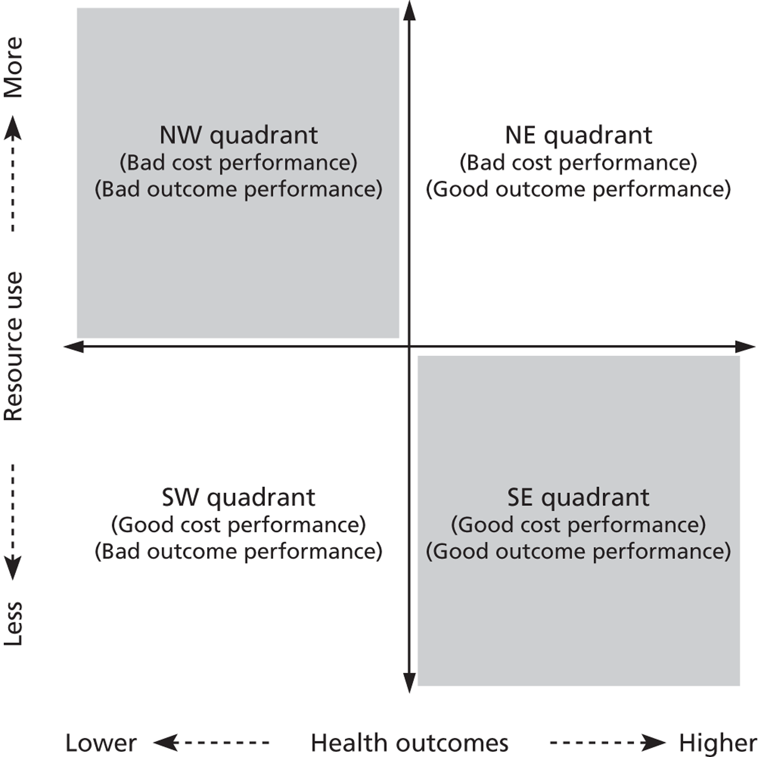
Hospitals can be classified into four different groups according to their performance on these two objectives: better or worse than expected performers on both objectives simultaneously, or better or worse than expected performers on one objective, but not the other. Hospitals located in the north-east and south-east quadrants of the plane are identified as better than expected (‘good’) performers in terms of health outcomes, whereas those in the two western quadrants are seen as worse than expected (‘poor’) performers with respect to this objective. The same principle applies to their resource use, where all hospitals in the southern quadrants perform well, whereas those in the northern quadrants perform badly, utilising more resources than expected. A hospital is identified as performing well on both objectives if it is situated in the south-east quadrant and provides care using substantially fewer resources and achieves higher health outcomes than expected given their case mix and production constraints. Hospitals located in the north-west quadrant are considered to perform badly with respect to the two objectives as they deliver poorer outcomes and utilise more resources than expected.
Our second set of empirical analyses focuses on these issues and is discussed below.
Chapter 3 Data sources
In order to perform our empirical analyses, our study combines data from the English Hospital Episode Statistics (HES) inpatient database with the PROMs survey and the reference cost (RC) databases for the period April 2009 to March 2010. The HES database includes detailed information on all NHS-funded inpatient care provided by public and independent sector hospitals in England. We extract data on all elective patients, aged 15 years or over, who underwent unilateral hip or knee replacement, varicose vein surgery or groin hernia repair. Each patient is defined in terms of the duration of his or her hospital stay (termed, in England, as an inpatient spell). One of the idiosyncrasies of the HES database is the recording of inpatient activity at consultant level. When multiple consultants treat a patient, more than one Finished Consultant Episode (FCE) is generated. This is typically the case when patients require multidisciplinary care and are transferred between specialties within the same hospital. In order to record all relevant information regarding admission, discharge or comorbidities and to keep in line with international literature on hospital activity, we link all FCEs arising from admission to discharge to construct inpatient spells. 29 We retain only complete records for each patient, i.e. where all relevant information is recorded. Duplicate observations are removed from the database according to the algorithm described in Appendix 1 .
Since 2009, patients having one of four common surgical procedures have been surveyed about their health status before and after treatment. The four procedures are unilateral hip replacement, unilateral knee replacement, varicose vein surgery and groin hernia repairs. 2 All providers of publicly funded inpatient care in the English NHS are required to offer the pretreatment survey to all their patients who pass as fit to have one of these procedures. There may be systematic differences among hospitals in how many of their patients are surveyed, especially if hospitals differ in the process by which they offer and administer the survey. Patients are surveyed again, either 3 or 6 months post surgery, depending on the procedure. This post-treatment survey is administered at a national level by an organisation contracted by the Department of Health. For individual patients, we link the PROM surveys to the HES data using the episode identifier epikey. This linkage allows us to take account of a range of patient characteristics when we analyse the PROMs data and to assess whether patients who responded to the pre- and post-treatment PROM surveys differ from those that did not respond.
Cost data are linked to the HES data based on the Healthcare Resource Group (HRG), to which the patient has been allocated, the hospital and specialty identifier, his or her admission type and his or her length of stay (LoS). For more detailed information on how to link HES and cost data, see the study by Laudicella et al. from 2010. 30
Health outcomes
We measure a patient’s health status before and after surgery using condition-specific PROMs as well as a generic measure, the EQ-5D. Data are derived as part of the PROM survey, where all eligible patients undergoing one of the four elective procedures are invited to participate. 2 Table 1 provides an overview of the PROMs that are collected as part of the national PROM programme. Patients that have consented to participate are requested to complete the paper-based survey prior to surgery. These data are usually collected during the last outpatient appointment preceding the surgery or on the day of admission. As noted above, patients are then sent another questionnaire either 3 or 6 months post surgery via postal mail. To ensure consistency with respect to the timing of measurements, while retaining as much information as possible, we exclude all observations for which (1) the recorded time between the pretreatment survey and admission exceeds 12 weeks, (2) the post-treatment period is either shorter than 20 weeks or longer than 1 year for hip replacement and knee replacement patients, and (3) the post-treatment period is either shorter than 8 weeks or longer than 24 weeks for groin hernia and varicose vein surgery patients.
| Procedure | Condition-specific PROM | Generic PROM | Data collection time (months post operation) |
|---|---|---|---|
| Knee replacement | OKS | EQ-5D (including EQ-VAS) | 6 |
| Hip replacement | OHS | EQ-5D (including EQ-VAS) | 6 |
| Varicose vein surgery | AVVQ | EQ-5D (including EQ-VAS) | 3 |
| Groin hernia repair | – | EQ-5D (including EQ-VAS) | 3 |
The EQ-5D is a generic measure of health-related quality of life. It consists of two components: the EQ-5D descriptive system and a visual analogue scale, the EQ-VAS. The EQ-5D descriptive system is a widely used generic measure of health-related quality of life. 10,31 It describes impairments in overall health through self-assessed limitations on five dimensions: mobility, self-care, usual activities, pain/discomfort and anxiety/depression. For each of the five dimensions, patients can indicate whether they have (1) no problems, (2) some/moderate problems or (3) extreme problems (in the case of the pain/discomfort and anxiety/depression), are unable to (self-care and usual activities) or are confined to bed (mobility). Responses on each dimension are translated into numeric values ranging from 1 to 3. A patient’s health profile can then be described as a series of numerical values, e.g. 11221 representing a patient that has some problems performing usual activities and experienced moderate pain/discomfort, but reports no problems regarding any other health dimension.
The EQ-5D health profile can be aggregated to an index score using a UK-specific set of weights that are derived from the general public and reflect societal preferences. 11 The resulting index scores range from – 0.542 to 1, where 1 is defined as perfect health and 0 is defined as equivalent to being dead. Values lower than 0 indicate health states that are considered worse than being dead. 32 Following the discussion in Chapter 2 , we use data on the health profile of the patient to analyse hospital impact on individual dimensions of health and the EQ-5D utility index to assess hospital performance in terms of cost of treatment and outcomes.
The EQ-5D is a two-part instrument that also contains a vertical EQ-VAS. The EQ-VAS can be used to elicit the patient’s own valuation of his or her own global health status. This scale ranges from 0 (worst imaginable health) to 100 (best imaginable health). Patients indicate their current level of health by drawing a line from a box outside the rating scale to a point on the scale that reflects their current health state. The EQ-VAS is the only measure collected as part of the PROM programme that does not require aggregation of multiple dimensions of questionnaire items into an index score. This allows us to analyse responses to this instrument without making any adjustments to the reported values.
The condition-specific instruments are the Oxford Hip Score (OHS), the Oxford Knee Score (OKS) and the Aberdeen Varicose Vein Questionnaire (AVVQ). The OHS and OKS each comprise 12 questions that reflect limitations in health-related quality of life brought about by the either the hip or the knee joint. 33,34 Responses to each question are recorded on an ordinal scale ranging from 0 to 4, where 0 indicates several problems and 4 indicates no problems. An overall score is calculated by weighting questions equally and summing all answers. Accordingly, the overall scores range from 0 (worst) to 48 (best). The AVVQ contains 13 questions which can also be aggregated into an index score. 35 This index score lies between 0 and 100, with higher numbers indicating worse health states; however, in order to facilitate interpretation and comparison of estimation results, we recode the AVVQ scores so that they range from 0 (worst) to 100 (best). No condition-specific PROM is collected for groin hernia repair.
As patients complete both components of the EQ-5D and the relevant condition-specific measure, we are able to explore whether or not results are sensitive to the choice of PROM instrument. These sensitivity analyses are intended to provide insight into which PROM instrument should be used to measure outcomes. For the comparative analysis reported in The relationship between costs and outcomes, we include only observations for which the full set of PROMs was completed.
Resource use
Resource use is measured as either inpatient costs or LoS. We derive information on hospital costs from the RC database, which is an annual compilation of cost data that forms the basis for the calculation of reimbursement tariffs under Payment by Results36 and whose completion is compulsory for all NHS-operated hospitals. 37 LoS is derived directly from HES.
Reference costs are measured using a top-down costing methodology. The NHS Costing Manual 37 sets out rules to ensure that costs are matched as closely as possible to the services that generate them and to maximise direct attribution of costs in preference to apportionment. Costs are calculated on a full absorption basis, meaning that they should reflect the full cost of the service delivered and have to reconcile back to the general ledger. Total hospital costs are assigned to increasingly more granular levels of a hierarchy of costing centres; beginning at treatment services, to specialties and then to individual HRGs. Costs at the HRG level are reported separately by specialty and are further broken down by admission type (day case, elective and emergency care) and LoS, where HRG-specific trim points are used to differentiate short, usual and long inpatient spells. Our process of linking RC to HES records generates costs that are the most specific to an individual patient that can be achieved given the top-down cost allocation methods that are used by English hospitals.
All costs are adjusted for the market forces factor (MFF) specific to the hospital. 38 This adjustment takes into account the unavoidable variation in input prices across the country as defined by the Department of Health.
Costs are often preferred to LoS as a proxy of resource use because, in theory, they summarise the range of inputs utilised in the production process. However, the true costs of production are difficult to assess, particularly in terms of allocating shared inputs, and the reported RCs may be prone to measurement error. (We exclude one hospital from the analysis of cost and outcomes because of obviously incorrect RC data. The average cost of care in this hospital for the hip replacement patients in our sample was reported to be £79, which is impossible under all reasonable explanations. The hospital reported similarly unrealistic costs for the other three conditions.) LoS, while being a less comprehensive measure of resource use, is less likely to be affected by measurement error. We therefore explore the sensitivity of our results to the choice of resource use measure.
Observed patient characteristics and risk factors
We derive a generic set of risk-adjustment variables that reflect patient severity and are used to model both resource use and health outcomes for all four surgical procedures. This builds on the preliminary risk-adjustment methodology developed by the NHS Information Centre that was, until recently, applied to the PROM data. 9
The primary risk adjuster is the patient’s self-reported health status before surgery, i.e. the pretreatment PROM. We argue that this captures information about an individual patient that could not be captured by the other observable characteristics in the HES dataset (e.g. age, gender, etc.). For example, we may know that older patients in general may have lower outcomes or higher costs, but knowing a patient’s specific pretreatment PROM allows far greater scope in understanding the expectations for this particular patient. The ability to use pretreatment PROM scores as a risk-adjusting variable is thus a major advance in risk adjustment.
In addition, we also extract information on age, gender and number and type of comorbidities [International Classification of Diseases – Tenth Edition (ICD-10)] from the HES inpatient dataset. The number and type of comorbidities are used to account for the number of additional diagnoses coded and to construct the weighted Charlson index;39 6 of the 17 Charlson comorbidities are designated as severe and given greater weight than the other eleven. 40 We also record whether the patient underwent revision surgery (based on Office of Population Censuses and Surveys procedure classification, version 4.5) or whether the patient was treated by multiple consultants during his or her hospital stay. The patient’s socioeconomic status is approximated by the income deprivation profile of the neighbourhood in which the patient resides [i.e. the Index of Multiple Deprivation (IMD)].
We also construct indicator variables for the five most common HRGs to which patients are allocated and group all other observations in the category ‘other’. HRGs are, by design, homogeneous with respect to the expected level of resource utilisation. They are, therefore, expected to explain a majority of variation in observed cost of treatment or LoS. In contrast, HRGs are not designed or validated to categorise risk profiles with respect to health outcomes. We therefore include HRG dummies in the resource use equations but not in the outcome equations.
Finally, we derive two variables that are expected to reflect hospital production constraints. We calculate the number of patients treated for each of the four conditions by each hospital. Volume has been identified as one potential driver of resource use and health outcomes. 41 Given the excess demand faced by most English NHS hospitals, we expect volume to be outside the hospitals’ control, at least in the short term and, therefore, we adjust all performance estimates accordingly. Hospitals may also face production constraints because of existing teaching commitments. We therefore categorise hospitals into teaching and non-teaching facilities based on the classification system adopted by the National Patient Safety Agency. 42
Missing data
Participation in the PROM survey is mandatory for hospitals, but optional for patients. As such, one would expect that some eligible patients do not participate and health status measures are missing. This may be because patients either did not complete the pretreatment survey (both data points are missing) or patients were lost to follow-up (one data point is missing). This raises the questions (1) whether the patients for whom PROM data are missing differ systematically from those who provided data and (2) whether there are systematic differences among hospitals with regard to the type of patients have missing data.
The key to dealing with missing data is to understand the mechanism that drives the ‘missingness’ and the differing consequences that follow. There are, generally argued to be, three missing data mechanisms:43,44
-
Missing completely at random (MCAR): missing data have no systematic relationship to the value of any other observed or unobserved variables or the value of the missing data item itself. The mechanism that drives the missingness is purely exogenous and has no implications for the analysis other than that it reduces sample size.
-
Missing at random (MAR): missing data may be systematically related to the value of other observed variables (e.g. data for males are less likely to be missing), but conditional on those values, the data are MCAR. In other words, the data about the outcomes for males that we do observe are representative of the outcomes for males we do not observe. The important aspect in this case is that the missing values are related to observable characteristics of individual patients, not to characteristics that are unobserved.
-
Missing not at random (MNAR): missing values may occur because of the value of the missing data item itself or other unobserved characteristics. Effectively, the patients we do observe for a particular hospital may not be representative of the patients who we do not observe. If, for example, sicker patients were less likely to fill out post-treatment questionnaires, then the mean health outcome observed for any particular hospital would be an overestimate.
Missing data pose substantial problems for any type of analysis. The problem is that, by the very nature of the data being missing, it is virtually impossible to determine which type of missing mechanism is in operation. Indeed, even if one could be certain that the data are MAR, i.e. they are missing because of the value that a certain other variable takes, one can rarely provide conclusive evidence for them not being MNAR. In this sense, the problem of missingness can only truly be overcome by actually collecting the missing data.
Our study is a secondary data analysis and resources were not available to collect primary data. We therefore adopt two strategies to address the issue of missing data. First, we report characteristics of patients who did or did not provide data to allow readers to assess the degree of missingness and come to a judgement about the data-generating mechanism at work. Second, the analysis reported in Identifying variation in patient-reported outcomes across hospitals makes use of the unique data structure and analytical techniques developed in the context of multilevel modelling to condition observed patient characteristics for those patients who have at least provided pretreatment health status information, and analyse the data under the less restrictive MAR assumption. Observations for which both data points are missing are still treated as MCAR.
The analysis reported in The relationship between costs and outcomes operates under the assumption of MCAR for both pre- and post-treatment health status data owing to constraints imposed by the analytical model.
Chapter 4 Analysis
Based on the two research questions developed in Chapter 2 of this report, we develop different statistical approaches to assess hospital performance with respect to, first, their ability to promote PROs and, second, to balance the pursuit of outcomes and cost control. The two research questions are pursued individually and are thus outlined separately.
Identifying variation in patient-reported outcomes across hospitals
Methodology and statistical approach
The objective of the first set of empirical analyses is to obtain estimates of the relative systematic impact of hospital providers on patients’ post-treatment health outcomes. We estimate hierarchical ordered probit models45–47 separately for each of the five dimensions in the EQ-5D questionnaire and then compare the results with those obtained from a linear regression on the EQ-5D utility scores to study the practical implications of using disaggregated health dimensions for assessment of hospital performance.
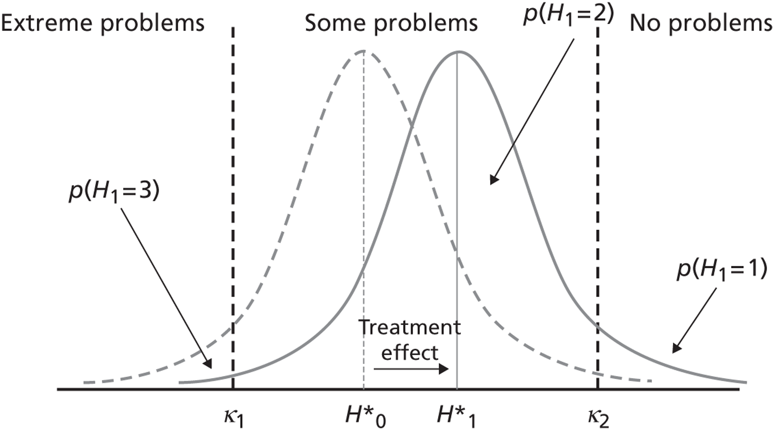
The intuition underpinning the ordinal model is that patient health status (with respect to a given dimension of the EQ-5D, e.g. pain/discomfort) is continuous, but cannot be directly observed. If health could be observed, one could directly measure the average effect of treatment and the variation in treatment effect between hospitals. However, because health is not observable, patients are asked to classify their underlying health according to a measurement model, leading to three possible classifications, i.e. no, some or extreme problems. This classification is based on cut-off points, which are also not directly observable but can be estimated from the data. For example, if a patient’s underlying health status is higher than cut-off κ 2, but lower than cut-off κ 1, then the patient will classify himself or herself as having ‘some problems’. This is depicted in Figure 2 . By assuming a probability distribution for the possible classifications and using the observed patient classifications, we can estimate the cut-off points and study movements between classifications brought about by treatment. This is shown in Figure 3 .
FIGURE 2.
The measurement model of self-reported health classification.
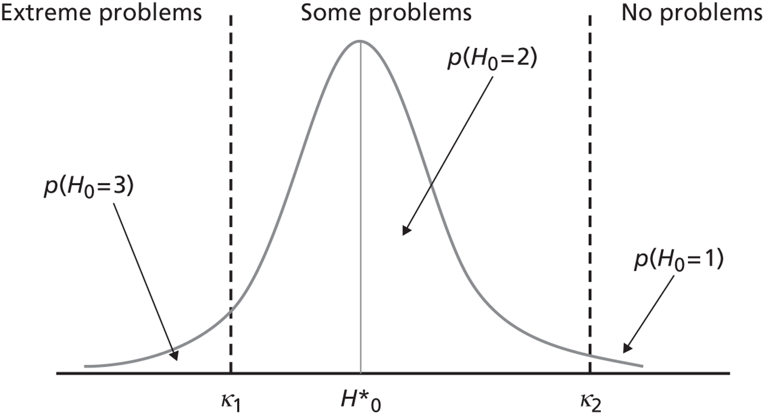
FIGURE 3.
Identifying treatment effects in self-reported health classification.
More formally, let H i j t * denote the health status of patient i = 1, . . ., n j in hospital j = 1, . . ., J at time point t ϵ [0,1]. Health status is assumed to be continuous and ranges from negative infinity to positive infinity. However, health status is not directly observable and, instead, we observe patients’ own assessment of their status on the three-point EQ-5D response scale (m = 1, 2, 3 with 1 = no problems, 2 = some problems, 3 = extreme problems). The mapping of underlying, continuous status H i j t * to observed, discrete health status category H ijt is given by the standard measurement model:48
where the threshold parameters, κ, are unobserved and must be estimated from the data. The categories are ordered from worst to best. This facilitates the qualitative interpretation of regression coefficients, where a positive sign indicates improvements in underlying health and, thus, the probability of reporting no problems.
Each patient provides measures of his or her health status pre and post treatment. Both responses are determined partly by common factors, such as patient characteristics and underlying health. Our interest lies in the change between pre- and post-treatment health status and the degree to which variation in this health outcome can be systematically associated with the hospital providing the care. We make the assumption, based on the conditional pretreatment health status of a patient and a set of risk-adjustment factors, that patients do not select hospitals based on unobservable characteristics and that the health of patients in different hospitals would follow the same trajectory if untreated. This allows us to interpret the variation in health outcome across hospitals as a measure of relative quality performance.
Our data are characterised by a hierarchical structure, with measurement points clustered in patients, which themselves are clustered in hospitals. Given the non-linear nature of our model, these data can be analysed in two ways. One can collapse the hierarchy into two levels and model post-treatment health status as a function of lagged, observed (pretreatment) response H ij 0, observed patient characteristics and a hospital effect. 49 The alternative way can treat both pre- and post-treatment health status as left-hand-side variables and estimate longitudinal models with unobserved patient heterogeneity. 47,50,51 We adopt the second approach because it allows us to (1) explicitly account for unobserved, time-invariant determinants of underlying health, (2) utilise information contained in both the pre- and post-treatment observations to estimate threshold parameters, (3) acknowledge heterogeneity in underlying health within a health status category as well as random error in reported pretreatment health, and (4) extend the model in a natural way should more measurement points become available in the future. 52 Furthermore, it allows us to incorporate information on patients who reported their health status prior to treatment but were subsequently lost to follow-up. The missing data for these patients are treated as MAR, an improvement over the MCAR assumption that underpins the two-level regression approach.
Health status at any time point t is described by the equation
with
The vector x ij is a set of patient-level risk-adjustment variables that are, in this case, time invariant, where beta (β) is the estimate of the influence of each variable. Treatment is modelled as a dummy variable T, which takes a value of 1 if t = 1 (post-treatment) and 0 otherwise. The direct effect of treatment on post-treatment health is given by the coefficient υ j . We also interact T with x ij to allow for differential effects of patient characteristics on pre-treatment health status and on the effect of treatment.
Unexplained variation is composed of four variance components: (1) a patient-specific intercept α i j ∼ N ( 0 , σ α 2 ) that captures unobserved, time-invariant patient heterogeneity in underlying health, (2) a hospital-specific, time-invariant intercept ζ j ∼ N ( 0 , σ ζ 2 ) that addresses hospital clustering, (3) a random coefficient γ j ∼ N ( 0 , σ γ 2 ) that varies between hospitals and describes the systematic hospital effect on post-treatment health and (4) a serially uncorrelated error term ε i j t ∼ N ( 0 , 1 ) that leads to the well-known probit specification. Covariance terms between random effects on the same level of the hierarchy are freely estimated, whereas terms across levels are constrained to zero. The variance partition coefficient τ describes the extent to which unexplained variation in post-treatment health occurs at the level of the hospital and is calculated as follows:53
Larger values of τ indicate that more variation in post-treatment health is attributable to variation among hospitals as captured in the hospital-level intercept ζ j and the random coefficient on treatment υ j .
For the EQ-5D utility model, we adapt our empirical model to a linear specification with an identity link function (i.e. H i j t * = H i j t ) and ε i j t ∼ N ( 0 , σ ε 2 ) .
Our interest lies in estimates of the relative quality of each hospital, γ j , captured by the hospital-specific deviation from the average effect of treatment, μ. This parameter is not directly estimated but can be evaluated in post-estimation using Bayes’ theorem with variance estimates entered for the unknown population parameters, which is a technique known as Empirical Bayes prediction. 54
The empirical Bayes estimates (EBEs) are estimated in two distinct steps. First, the risk-adjustment model is estimated using individual patient-level data while recognising the clustering of patients within hospitals. Secondly, using this distribution as an ‘empirical’ prior, we can then obtain hospital-specific estimates.
In the first step, the clustering is treated more as a data problem than as a parameter of interest and the systematic hospital effects are integrated out of the data in order to provide unbiased and precise estimates of the impact of the observed characteristics.
This first-step regression provides us with two important pieces of information. First, it gives us the means to quantify the expected impact of patient characteristics on outcomes and, thus, identify any hospital-level deviations not due to case mix. Second, it provides an estimate of the variance parameter σ γ 2 and hence the distribution γ j ∼ N ( 0 , σ γ 2 ) from which the hospital effects are assumed to be drawn. Using this distribution as an empirical prior, we can then obtain hospital-specific estimates, γ ^ j , in a second step by applying Bayes’ theorem; that is, the posterior distribution of an individual hospital effect γ j shown as
is a function of the likelihood of the observed outcomes, p ( H j | x . ; β ^ , γ j ) , i.e. the likelihood of observing outcomes, H j , in hospital, j, given the case mix, x .j , the estimated impact of the risk adjusters, β ^ and a random effect γ j , multiplied by the prior distribution of γ j , that is p ( γ j | x . ; β ^ ) .
It can be seen that where the posterior equation has a likelihood that dominates the prior, the random-effect estimate will be the same as the fixed-effect estimate, a scenario that would typically occur when sample sizes are large or random noise is small. Conversely, if sample sizes for each individual hospital are small, then there will be a divergence between the fixed- and random-effect estimates because the distribution of the likelihood implied by the data is different to that of the prior. More specifically, the random-effects model will produce estimates that are drawn towards the prior mean, zero, which is a process known as shrinkage. This can be interpreted as the estimated reliability of the fixed-effect estimate as a measure of γ j . 54 Alternatively, the random-effect estimate itself can be regarded as a precision-weighted estimate. 55
Based on estimates of γ j , we can now proceed to describe hospital performance. For non-linear models, we do this in two different ways. First, we rank hospitals according to their impact on latent post-treatment health status H i j 1 * . This can be directly inferred from γ ^ j , where a greater number of positive values indicate better performance. Second, we compute the probability of reporting a specific post-treatment health status category (m = 1, 2, 3), based on the estimated effort exerted by the hospital in providing high-quality care, as determined indirectly from the equations. For the average patient treated in a hospital of average patient intake, this is given by
where
and κ 0 = − ∞ , κ 3 = + ∞ . We calculate 95% credible intervals (CrIs) around γ ^ j based on their posterior distribution. Because our interest is on profiling hospital performance, we do not consider uncertainty in other parameter estimates when calculating CrIs for Prob(y j 1 = m).
Both methods produce identical rankings of relative hospital performance. However, only the second method relates the result back to the original scale of the PRO survey instrument and allows differences across hospitals to be investigated in terms of the probability of achieving a specific health outcome.
For the linear model on the EQ-5D index values, we rank hospitals directly on the basis of estimates of γ j .
All ordered probit models are estimated by maximum likelihood using Generalised Linear Latent and Mixed Models computer package (GLLAMM) in Stata 12 (StataCorp LP, College Station, TX, USA), where the integrals for the random effects are approximated by adaptive quadrature. 56 Threshold parameters and the scale of the coefficient are identified through constraints on the mean and variance of the error term and the mean of the intercept. The linear EQ-5D utility model is estimated by maximum likelihood using xtmixed in Stata 12.0.
Descriptive statistics
Patient level
Our sample consists of 27,133 patients having a hip replacement in a total of 154 NHS and private hospitals. The number of patients in each hospital ranges from 1 to 1212 [mean = 176, standard deviation (SD) = 148]. A total of 79.8% (n = 21,645) of these patients provide a complete EQ-5D health profile both pre and post treatment. The remaining 20.2% (n = 5488) only provide a complete pretreatment EQ-5D health profile. We present descriptive statistics of patient characteristics in Table 2 .
| Variable | Description | Mean/% | SD | Minimum | Maximum |
|---|---|---|---|---|---|
| male | = 1,a if patient is male | 41.7% | 0.49% | 0 | 1 |
| age | Patient’s age (years) | 67.41 | 11.40 | 15 | 96 |
| wcharlson | Weighted Charlson index of comorbidities | 0.32 | 0.67 | 0 | 8 |
| add_diagnoses | Number of additional diagnoses not included in Charlson index | 1.94 | 1.85 | 0 | 18 |
| revision_complications | = 1,a if revision surgery because of complication with existing implant (ICD-10: T84)57 | 6.7% | 0.25% | 0 | 1 |
| revision_other | = 1,a if revision surgery for other reasons | 1.0% | 0.10% | 0 | 1 |
| osteoarthritis | = 1,a if main diagnosis is osteoarthritis (ICD-10: M15–19)57 | 86.4% | 0.34% | 0 | 1 |
| rheumatoid_arthritis | = 1,a if main diagnosis is rheumatoid arthritis (ICD-10: M05–06)57 | 0.5% | 0.07% | 0 | 1 |
| other_maindiag | = 1,a if main diagnosis is not osteoarthritis or rheumatoid arthritis | 6.0% | 0.24% | 0 | 1 |
| deprivation | IMD, income domain58 | 0.13 | 0.10 | 0.01 | 0.83 |
| pretest | Time between preoperative assessment and admission (days) | 19.82 | 18.84 | 0 | 84 |
| post-test | Follow-up (days) | 207.16 | 29.81 | 140 | 365 |
| n | Total number of patients | 27,133 | |||
| J | Hospitals | 154 |
Elective hip replacement surgery is performed predominantly on elderly patients (the mean age of patients = 67.4 years, SD = 11.4 years), with osteoarthritis being the most common reason for surgical intervention. The majority of patients in our sample are female (58.3%) and 7.6% of patients are admitted for revision surgery. The average time elapsed between preoperative assessment and date of admission is 20 days (SD = 18.8 days) and the mean follow-up period is 207 days (SD = 29.8 days).
Table 3 presents the transition matrices for each of the five dimensions in the EQ-5D. For usual activities, 12,652 (8842 + 1395 + 2415) patients report improvements in mobility after treatment, 761 (289 + 24 + 448) report deteriorations after treatment and 8963 (1065 + 7340 + 558) report no change. Table 3 also reports the pretreatment health status for patients who did not provide a post-treatment follow-up measure, but we do not consider them in the following discussion.
| Pretreatment | Post-treatment | ||||
|---|---|---|---|---|---|
| No (= 1) | Some (= 2) | Extreme (= 3) | No follow-up | Total | |
| Mobility | |||||
| I have no problems in walking about (= 1) | 1218 | 257 | 0 | 171 | 1646 |
| I have some problems in walking about (= 2) | 11,030 | 9769 | 14 | 4535 | 25,348 |
| I am confined to bed (= 3) | 17 | 68 | 4 | 50 | 139 |
| Total | 12,265 | 10,094 | 18 | 4756 | 27,133 |
| Self-care | |||||
| I have no problems with self-care (= 1) | 9076 | 929 | 13 | 1629 | 11,647 |
| I have some problems with self-care (= 2) | 7868 | 4210 | 72 | 2910 | 15,060 |
| I am unable to wash or dress myself (= 3) | 78 | 155 | 54 | 139 | 426 |
| Total | 17,022 | 5294 | 139 | 4678 | 27,133 |
| Usual activities | |||||
| I have no problems with performing my usual activities (= 1) | 1065 | 289 | 24 | 206 | 1584 |
| I have some problems with performing my usual activities (= 2) | 8842 | 7340 | 448 | 3198 | 19,828 |
| I am unable to perform my usual activities (= 3) | 1395 | 2415 | 558 | 1353 | 5721 |
| Total | 11,302 | 10,044 | 1030 | 4757 | 27,133 |
| Pain/discomfort | |||||
| I have no pain/discomfort (= 1) | 148 | 44 | 1 | 37 | 230 |
| I have some pain/discomfort (= 2) | 7482 | 5029 | 245 | 2320 | 15,076 |
| I am extreme pain/discomfort (= 3) | 3923 | 4686 | 652 | 2566 | 11,827 |
| Total | 11,553 | 9759 | 898 | 4923 | 27,133 |
| Anxiety/depression | |||||
| I am not anxious/depressed (= 1) | 11,878 | 941 | 60 | 2226 | 15,105 |
| I am moderately anxious/depressed (= 1) | 5635 | 2471 | 199 | 2155 | 10,460 |
| I am extremely anxious/depressed (= 3) | 492 | 451 | 163 | 462 | 1568 |
| Total | 18,005 | 3863 | 422 | 4843 | 27,133 |
Several interesting observations can be made from these data. First, the number of patients improving after treatment varies greatly by the health dimension under consideration. The dimension most improved after treatment is pain/discomfort, where 72.4% [(7482 + 3923 + 4686)/(11,553 + 9759 + 898)] of the patients in our sample report improvements as indicated by a transition to a more favourable category. This is consistent with clinical expectations and the general understanding that pain reduction (and improvements in physical function) is the most important outcome for hip replacement patients. 59 In contrast, only 29.5% [(5635 + 492 + 451)/(18,005 + 3863 + 422)] of patients report improvements from one category to another on the anxiety/depression dimension.
Second, the idiosyncratic labelling of the mobility question is clearly reflected in the distribution of pre- and post-treatment scores. 60,61 Of those reporting both pre- and post-treatment health status, only 89 (17 + 68 + 4) patients report being confined to bed prior to treatment, further reducing to 18 after treatment.
Finally, for each of the five dimensions, a considerable number of patients report no problems prior to treatment. This is especially pronounced on the dimensions self-care and anxiety/depression where 44.6% [(9076 + 929 + 13)/(17,022 + 5294 + 139)] and 57.8% [(11,878 + 941+ 60)/(18,005 + 3863 + 422)] of patients fall into this category, respectively. A total of 6.6% [(1218 + 257 + 0)/(12,265 + 10,094 + 18)] of patients report no problems prior to treatment with respect to mobility. Overall, 64 patients report having no problems with respect to any of the EQ-5D dimensions.
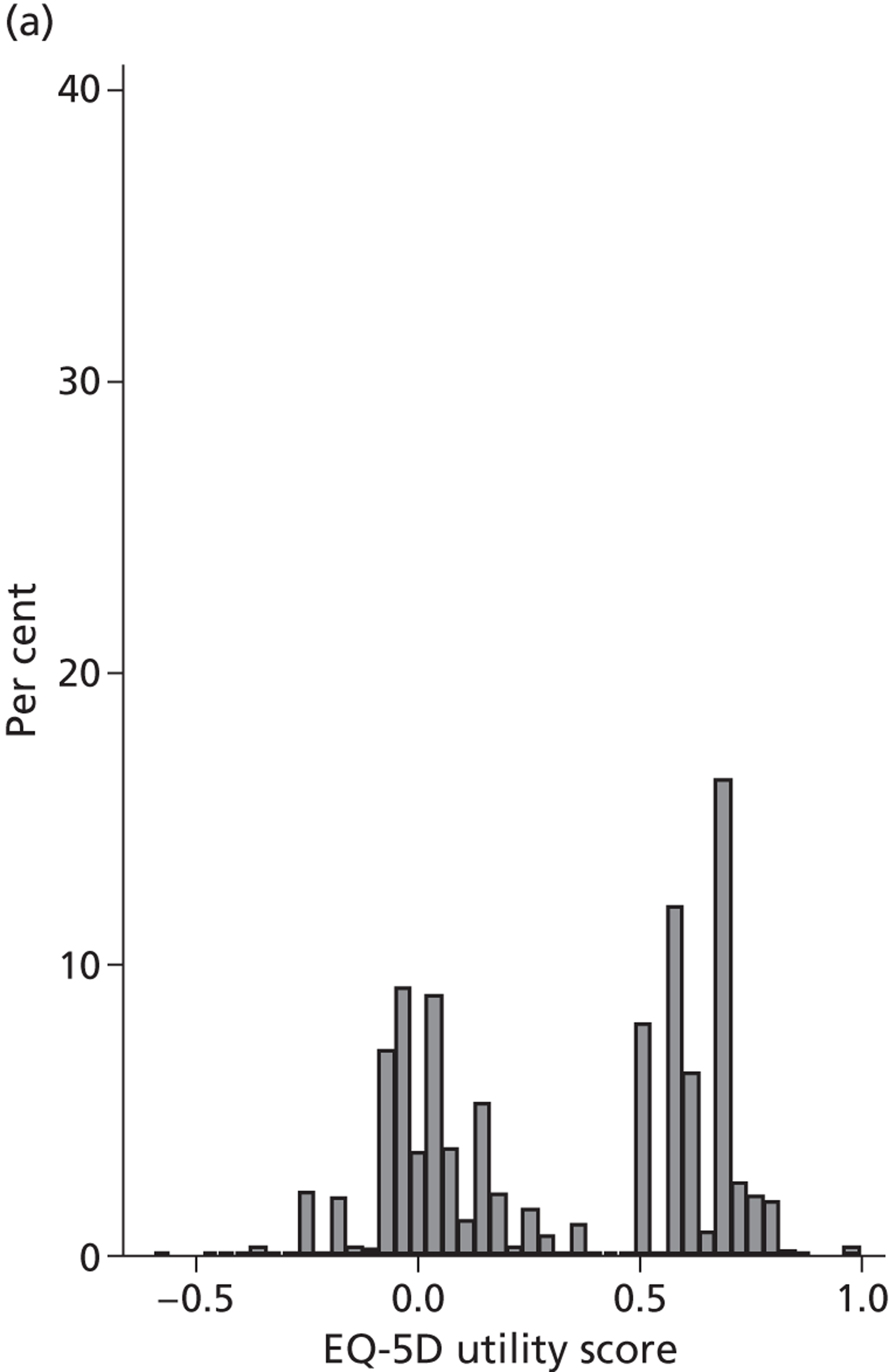
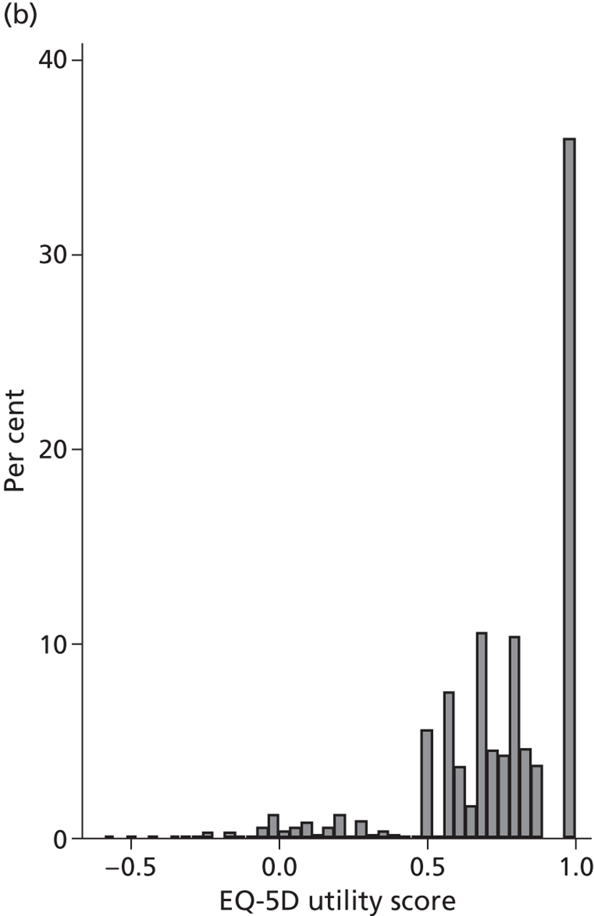
Figure 4 presents the empirical distribution of both the pre- and post-treatment EQ-5D utility scores. We focus on patients who have reported their health status at both occasions. The mean pretreatment score is 0.354 and the mean post-treatment score is 0.764. Both distributions exhibit typical characteristics of empirical EQ-5D distributions observed for a wide range of medical conditions, including multimodality, discontinuity and clustering at 1 (‘full health’). 18,19 A total of 87.3% of patients report improvements in health as measured by the EQ-5D utility index, whereas 6.4% report deteriorations.
FIGURE 4.
Distribution of the EQ-5D utility scores before and after hip replacement surgery. (a) Pretreatment; and (b) post-treatment.
Hospital level
Figure 5 shows hospital-level proportions of patients reporting each of the three potential responses (m = 1, 2, 3, i.e. no, some, extreme problems) for each dimension ordered by decreasing levels of patients reporting no problems. The pre- and post-treatment graphs for each dimension are shown side by side to demonstrate the unadjusted changes in pretreatment to post-treatment health status.
FIGURE 5.
Cumulative proportions of patients reporting a given level of health, by hospital.
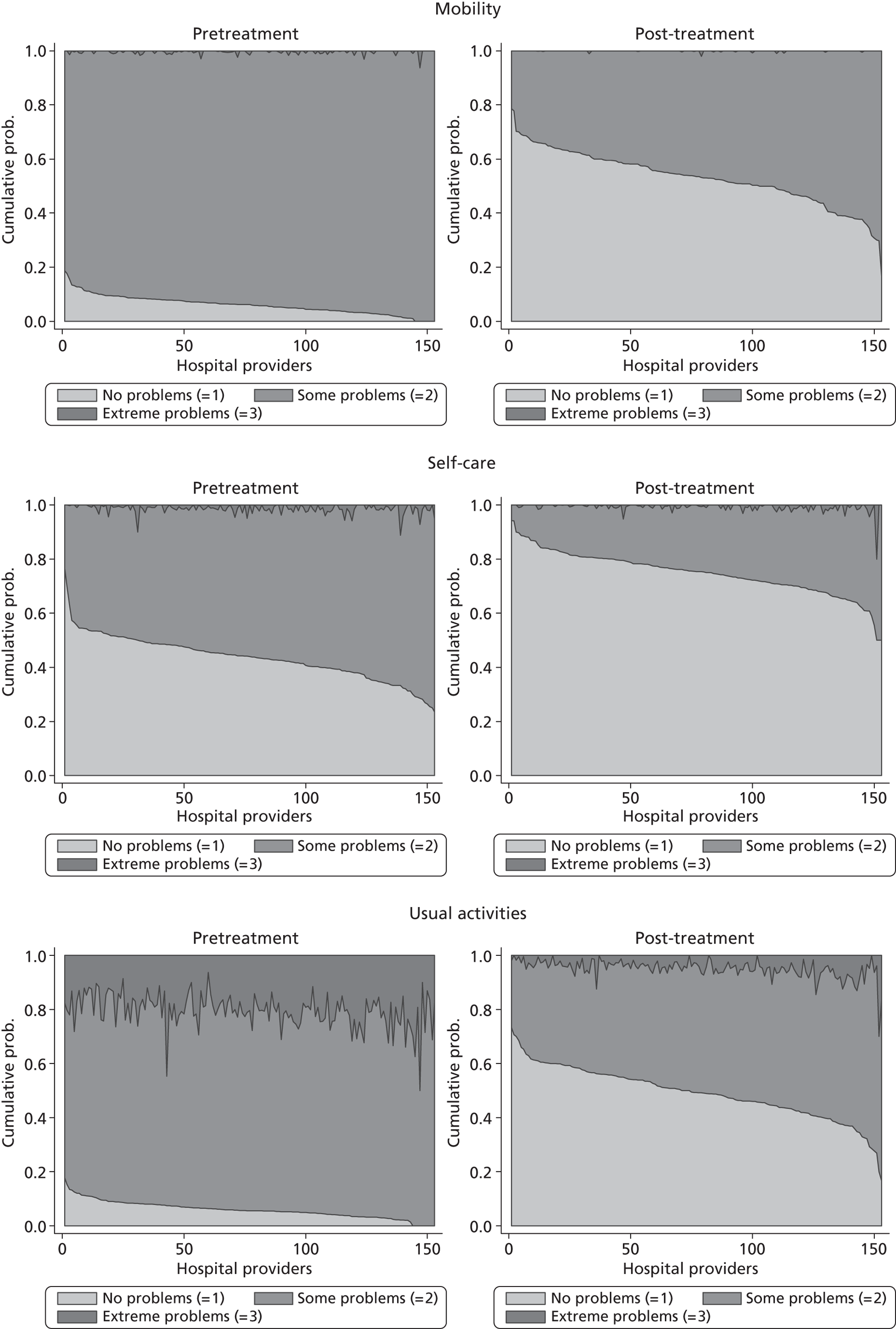
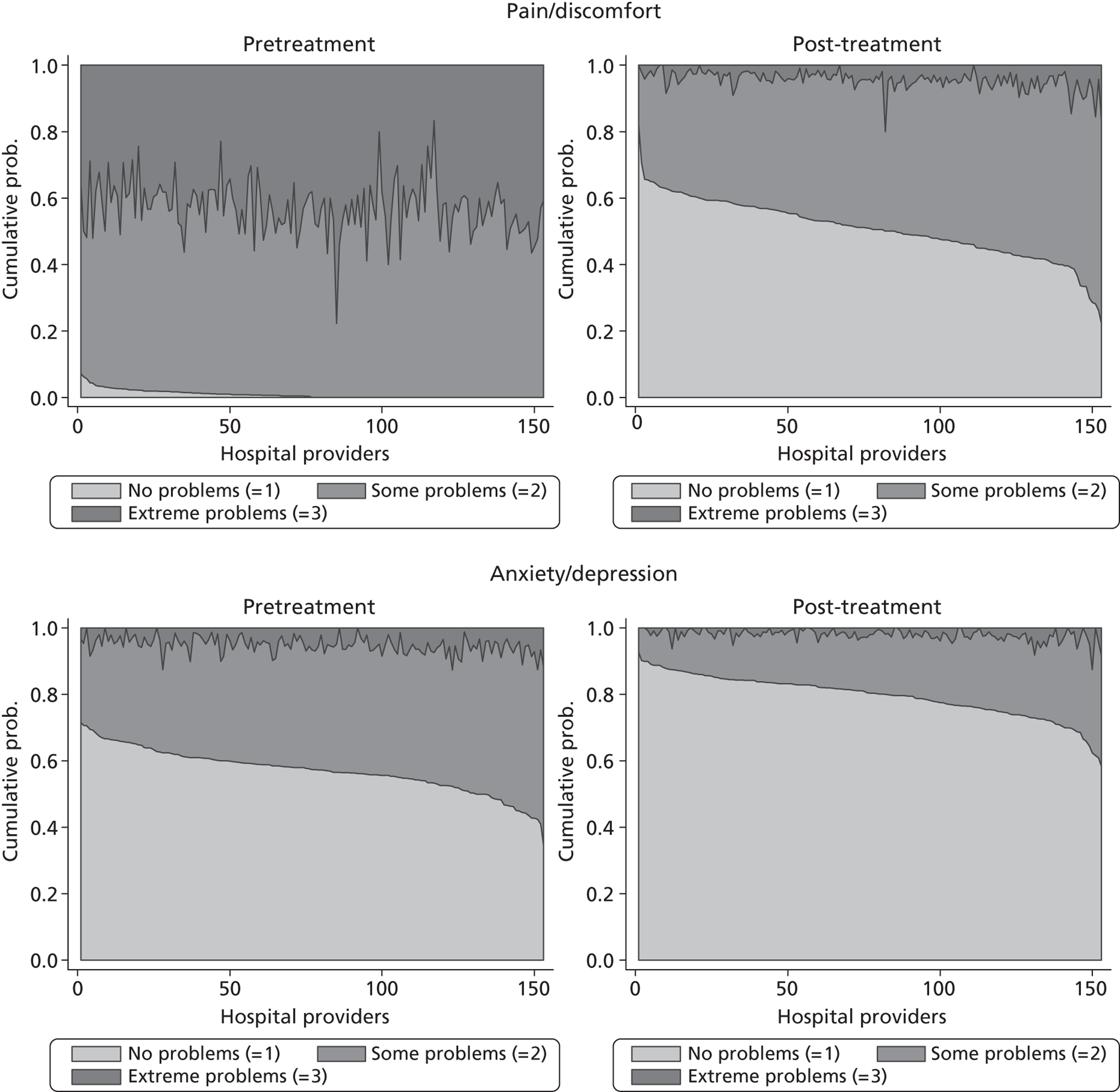
The following features are of interest. First, in all dimensions, there is a distinct improvement in average patient health outcome. This is most clearly indicated by the increase in the proportion of ‘no problems’ (lightly shaded areas) in the post-treatment (right-hand side) graphs. This is most notable for the mobility, usual activities and pain/discomfort dimensions.
Second, and correspondingly, there are large areas of pretreatment ‘extreme problems’ (darkest shaded areas) scores that do not appear post-treatment. This is most evident for usual activities and pain/discomfort.
Third, consider the slope of the boundary between the ‘no problem’ and ‘some problem’ areas for the post-treatment graphs. This pronounced slope indicates that there is the variation across hospitals in the proportion of patients in these two categories for all five dimensions. This occurs regardless of the amount of pretreatment variation.
This variation across hospitals requires investigation to determine whether it is due to the different characteristics of patients treated in these hospitals or is due to the performance of the hospital itself.
Missing data
Table 4 presents a comparison of patient characteristics across three groups of patients, those that provided health status measures either (1) at both pre- and post-treatment, (2) only at pretreatment or (3) never. The group means for each characteristic are compared by one-way analysis of variance method with Welsh’s test for unequal variances.
| Variablea | Not reported or excluded [mean (SD)] | Pretreatment only [mean (SD)] | Pre- and post-treatment [mean (SD)] | p-value |
|---|---|---|---|---|
| male | 0.40 (0.49) | 0.41 (0.49) | 0.42 (0.49) | 0.000 |
| age | 68.57 (11.73) | 65.95 (13.78) | 67.79 (10.69) | 0.000 |
| wcharlson | 0.35 (0.73) | 0.39 (0.77) | 0.30 (0.64) | 0.000 |
| add_diagnoses | 2.11 (1.97) | 2.19 (2.04) | 1.87 (1.79) | 0.000 |
| revision_complications | 0.12 (0.32) | 0.09 (0.28) | 0.06 (0.24) | 0.000 |
| revision_other | 0.02 (0.14) | 0.01 (0.11) | 0.01 (0.1) | 0.000 |
| osteoarthritis | 0.79 (0.41) | 0.83 (0.37) | 0.87 (0.33) | 0.000 |
| rheumatoid_arthritis | 0.01 (0.08) | 0.01 (0.09) | 0.00 (0.07) | 0.018 |
| other_maindiag | 0.08 (0.27) | 0.07 (0.25) | 0.06 (0.23) | 0.000 |
| deprivation | 0.13 (0.1) | 0.15 (0.11) | 0.12 (0.09) | 0.000 |
| n | 39,699 | 5488 | 21,645 |
There are statistically significantly differences for patient medical and demographic characteristics across groups, as would be expected given the large sample size. Patients who answer both pre- and post-treatment surveys, on average, have fewer comorbidities and a lower weighted Charlson score, are less likely to undergo revision surgery and are more likely to have a primary diagnosis of osteoarthritis. However, these differences are generally small and, arguably, of limited clinical significance.
Effect of observed patient characteristics on post-treatment health status
Table 5 presents parameter estimates and associated standard errors (SEs) for each of the five dimension models and the EQ-5D utility index model.
| Variablea | Mobility | Self-care | Usual activity | Pain/discomfort | Anxiety/depression | EQ-5D utility index | ||||||||||||
|---|---|---|---|---|---|---|---|---|---|---|---|---|---|---|---|---|---|---|
| β | SE | β | SE | β | SE | β | SE | β | SE | β | SE | |||||||
| male | 0.20 | 0.03 | *** | 0.01 | 0.02 | 0.09 | 0.02 | *** | 0.30 | 0.02 | *** | 0.47 | 0.02 | *** | 0.07 | 0.00 | *** | |
| age_15–60 | 0.06 | 0.04 | – 0.15 | 0.03 | *** | – 0.06 | 0.02 | * | – 0.10 | 0.02 | *** | – 0.29 | 0.03 | *** | – 0.03 | 0.01 | *** | |
| age_71_80 | – 0.08 | 0.04 | * | 0.04 | 0.03 | – 0.04 | 0.02 | 0.02 | 0.02 | 0.03 | 0.03 | 0.00 | 0.00 | |||||
| age_80+ | – 0.27 | 0.06 | *** | – 0.32 | 0.04 | *** | – 0.33 | 0.03 | *** | – 0.10 | 0.03 | ** | – 0.09 | 0.04 | * | – 0.05 | 0.01 | *** |
| add_diagnoses | – 0.10 | 0.01 | *** | – 0.08 | 0.01 | *** | – 0.06 | 0.01 | *** | – 0.06 | 0.01 | *** | – 0.07 | 0.01 | *** | – 0.02 | 0.00 | *** |
| revision_complications | 0.15 | 0.06 | ** | – 0.06 | 0.04 | – 0.08 | 0.04 | * | 0.23 | 0.03 | *** | – 0.09 | 0.04 | * | 0.01 | 0.01 | ||
| revision_other | 0.01 | 0.15 | 0.02 | 0.11 | – 0.06 | 0.09 | 0.18 | 0.09 | * | – 0.19 | 0.11 | 0.02 | 0.02 | |||||
| deprivation | – 0.91 | 0.15 | *** | – 1.30 | 0.11 | *** | – 0.40 | 0.09 | *** | – 1.21 | 0.09 | *** | – 1.18 | 0.11 | *** | – 0.33 | 0.02 | *** |
| wcharlson | – 0.12 | 0.02 | *** | – 0.15 | 0.02 | *** | – 0.13 | 0.01 | *** | – 0.11 | 0.01 | *** | – 0.11 | 0.02 | *** | – 0.04 | 0.00 | *** |
| rheumatoid_arthritis | – 0.67 | 0.21 | ** | – 1.03 | 0.14 | *** | – 0.49 | 0.12 | *** | – 0.43 | 0.12 | *** | – 0.25 | 0.14 | – 0.14 | 0.02 | *** | |
| other_maindiag | – 0.12 | 0.06 | – 0.13 | 0.05 | ** | – 0.18 | 0.04 | *** | – 0.04 | 0.04 | – 0.14 | 0.05 | ** | – 0.03 | 0.01 | *** | ||
| pretest | 0.00 | 0.00 | 0.00 | 0.00 | ** | 0.00 | 0.00 | * | 0.00 | 0.00 | 0.00 | 0.00 | *** | 0.00 | 0.00 | * | ||
| treatment | 2.73 | 0.10 | *** | 1.67 | 0.10 | *** | 2.26 | 0.08 | *** | 2.61 | 0.08 | *** | 1.71 | 0.10 | *** | 0.50 | 0.01 | *** |
| treatment × male | 0.08 | 0.03 | * | 0.04 | 0.03 | 0.19 | 0.03 | *** | – 0.06 | 0.02 | * | – 0.17 | 0.03 | *** | – 0.04 | 0.01 | *** | |
| treatment × age_15–60 | – 0.04 | 0.05 | – 0.02 | 0.04 | – 0.07 | 0.03 | * | 0.02 | 0.03 | – 0.06 | 0.04 | 0.01 | 0.01 | |||||
| treatment × age_71–80 | – 0.04 | 0.04 | – 0.06 | 0.04 | – 0.15 | 0.03 | *** | 0.03 | 0.03 | 0.04 | 0.04 | – 0.01 | 0.01 | |||||
| treatment × age_80+ | – 0.27 | 0.06 | *** | 0.01 | 0.05 | – 0.22 | 0.04 | *** | 0.16 | 0.04 | *** | 0.09 | 0.05 | 0.01 | 0.01 | |||
| treatment × add_comorbidities | – 0.03 | 0.01 | ** | – 0.02 | 0.01 | ** | – 0.05 | 0.01 | *** | – 0.01 | 0.01 | * | – 0.04 | 0.01 | *** | 0.00 | 0.00 | |
| treatment × revision_complications | – 0.80 | 0.07 | *** | – 0.56 | 0.06 | *** | – 0.55 | 0.05 | *** | – 0.69 | 0.05 | *** | – 0.34 | 0.06 | *** | – 0.11 | 0.01 | *** |
| treatment × revision_other | – 0.51 | 0.18 | ** | – 0.82 | 0.14 | *** | – 0.48 | 0.13 | *** | – 0.65 | 0.12 | *** | – 0.49 | 0.14 | *** | – 0.12 | 0.02 | *** |
| treatment × deprivation | – 0.69 | 0.18 | *** | – 0.47 | 0.15 | ** | – 1.02 | 0.13 | *** | – 0.12 | 0.13 | – 0.57 | 0.15 | *** | 0.03 | 0.02 | ||
| treatment × wcharlson | – 0.10 | 0.03 | *** | – 0.08 | 0.02 | *** | – 0.06 | 0.02 | ** | – 0.03 | 0.02 | – 0.03 | 0.02 | 0.00 | 0.00 | |||
| treatment × rheumatoid_arthritis | – 0.37 | 0.26 | – 0.16 | 0.19 | – 0.34 | 0.17 | * | – 0.28 | 0.17 | – 0.01 | 0.20 | – 0.02 | 0.03 | |||||
| treatment × other_maindiag | 0.03 | 0.08 | 0.02 | 0.07 | 0.03 | 0.06 | – 0.08 | 0.05 | 0.01 | 0.07 | 0.01 | 0.01 | ||||||
| treatment × posttest | – 0.00 | 0.00 | *** | – 0.00 | 0.00 | ** | – 0.00 | 0.00 | *** | – 0.00 | 0.00 | ** | – 0.00 | 0.00 | *** | – 0.00 | 0.00 | *** |
| constant | NA | NA | NA | NA | NA | 0.40 | 0.01 | |||||||||||
| к 1 | – 3.51 | 0.07 | *** | – 3.44 | 0.05 | *** | – 1.12 | 0.03 | *** | – 0.32 | 0.03 | *** | – 2.52 | 0.04 | *** | NA | ||
| к 2 | 1.69 | 0.05 | *** | – 0.12 | 0.03 | *** | 1.54 | 0.03 | *** | 2.13 | 0.03 | *** | – 0.41 | 0.03 | *** | NA | ||
| σ2 ε | constraint to 1 | constraint to 1 | constraint to 1 | constraint to 1 | constraint to 1 | 0.06 | 0.00 | *** | ||||||||||
| σ2 α | 0.53 | 0.04 | *** | 1.05 | 0.04 | *** | 0.44 | 0.02 | *** | 0.29 | 0.02 | *** | 1.21 | 0.05 | *** | 0.02 | 0.00 | *** |
| σ2 ζ | 0.02 | 0.01 | *** | 0.03 | 0.01 | *** | 0.02 | 0.00 | *** | 0.02 | 0.00 | *** | 0.02 | 0.00 | *** | 0.00 | 0.00 | *** |
| σ2 γ | 0.02 | 0.01 | *** | 0.01 | 0.00 | * | 0.02 | 0.01 | *** | 0.01 | 0.00 | *** | 0.01 | 0.01 | *** | 0.00 | 0.00 | *** |
| cov(ζ,γ) | 0.00 | 0.01 | 0.00 | 0.00 | 0.00 | 0.00 | 0.00 | 0.00 | – 0.01 | 0.00 | * | 0.00 | 0.00 | *** | ||||
| τ | 0.027 | 0.016 | 0.029 | 0.018 | 0.010 | 0.001 | ||||||||||||
| Log-likelihood | – 20,676 | – 30,989 | – 36,399 | – 36,781 | – 32,952 | – 7,403 | ||||||||||||
We find several variables to be associated with a higher level of reported health status. Those variables that are negatively associated with higher health status include a higher weighted Charlson index score, a greater number of additional comorbidities, being aged 80 years or older (relative to age 61–70 years), having a main diagnosis other than osteoarthritis and the deprivation profile of the patient’s neighbourhood of residence. Variables that are positively associated with higher health status include being male and the reports provided by patients admitted for revision surgery tend to show better health status on mobility and pain/discomfort than those undergoing primary surgery, but tend to be worse with respect to anxiety/depression. Patients who responded to the pretreatment survey sooner, i.e. the time elapsed between survey and admission is greater, tend to report better health status, but the effect of this better health status is very small.
The mean effect of treatment on post-treatment health is positive and significant for all dimensions. We observe some variation in treatment effect that is associated with observed characteristics of the patient, as captured by the interaction terms. For example, the number of comorbidities and the indicators for revision surgery are negatively associated with the treatment effect, indicating that treatment is less beneficial for multimorbid or revision patients. Similarly, patients living in more deprived areas experience, on average, less improvement in health than those residing in higher income areas. The timing of the post-treatment survey response has a statistically significant, but small, effect and patients who provide a PRO after a delay indicate that treatment has less of an effect.
As shown in Table 5 , all variance components are statistically significant at the 95% confidence level, as confirmed by likelihood ratio tests. In contrast, only the covariance term in the anxiety/depression and EQ-5D utility models are statistically significant. Only about 1.0% (anxiety/depression) to 2.9% (mobility) of the unexplained variation in underlying health is estimated to be associated with the hospital itself.
Risk-adjusted hospital performance on individual EQ-5D dimensions
We now turn to the results of the hospital performance assessment. Figure 6 presents estimates of hospital performance on the underlying health scale (left-hand graphs) and the probability scale (right-hand graphs), where the latter is calculated for the average diagnoses. Figure 7 presents the results of the EQ-5D utility model, where performance is measured directly on the utility scale. Hospitals located to the left side of each graph perform better than those to the right. The probability of reporting ‘extreme problems’ after surgery is close to zero for all models. We refrain from reporting CrIs around these predicted probabilities to increase the readability of the graphs.
FIGURE 6.
Performance estimates on the latent health and outcome scale.
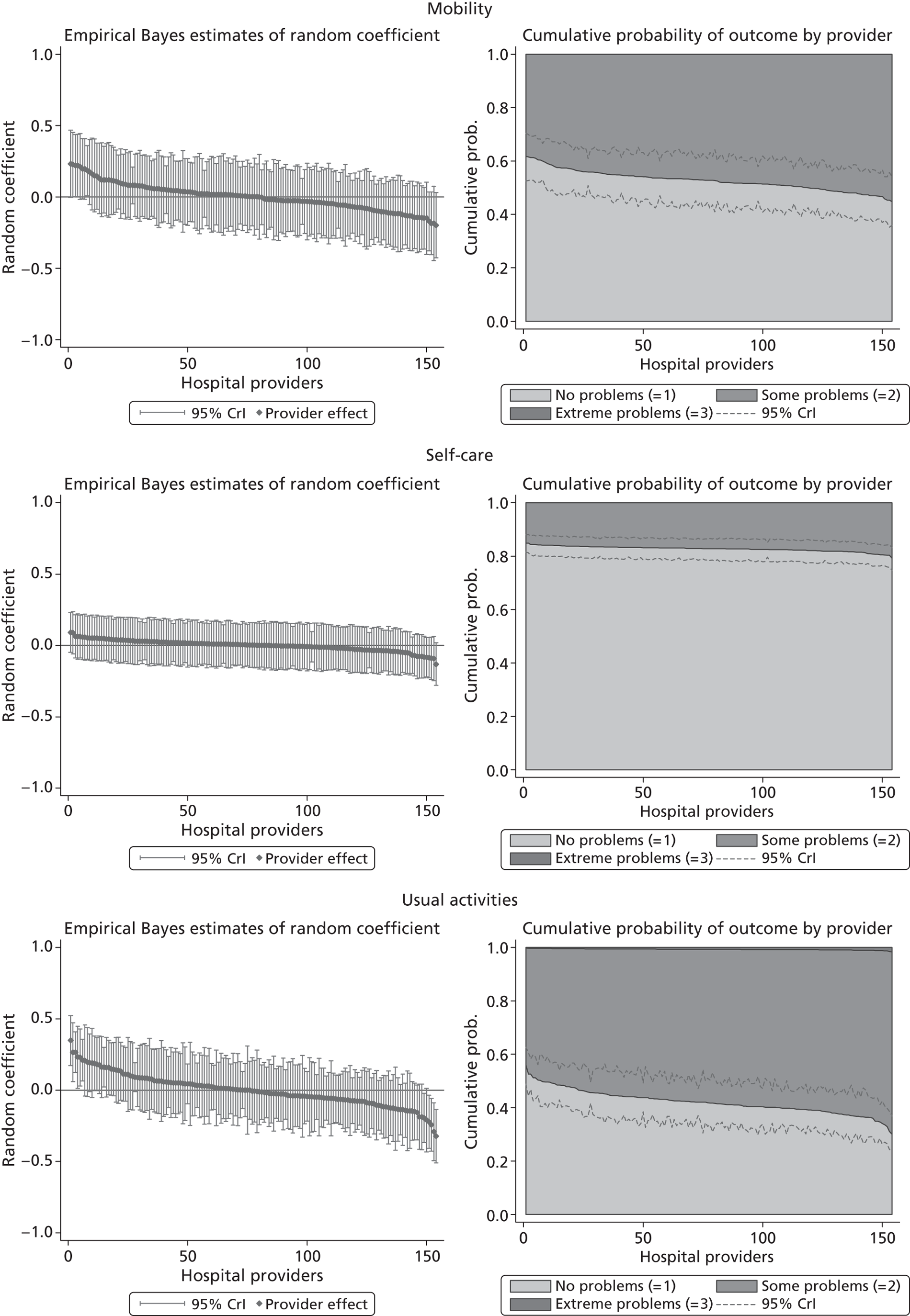
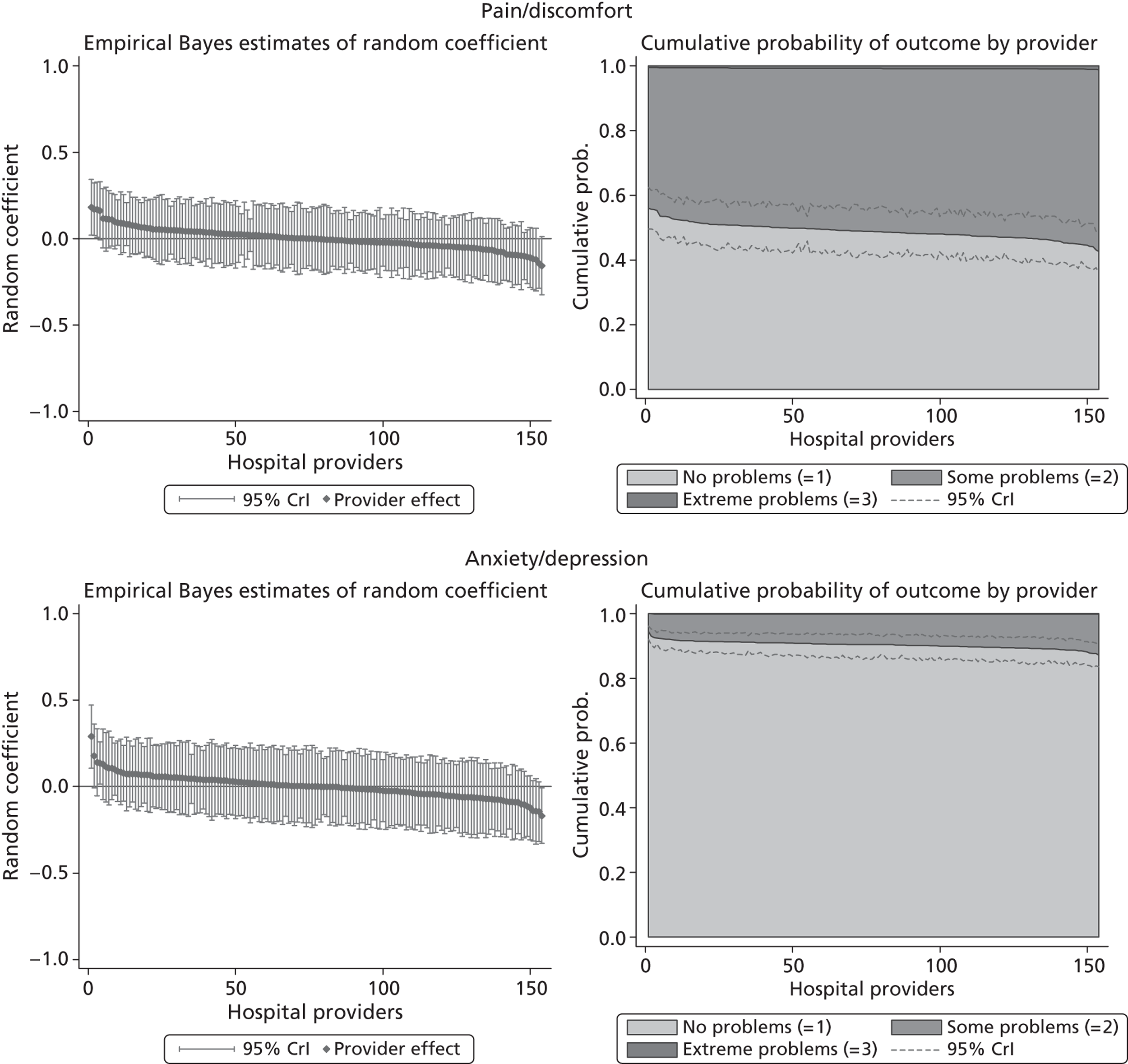
FIGURE 7.
Performance estimates on the overall EQ-5D utility scale.
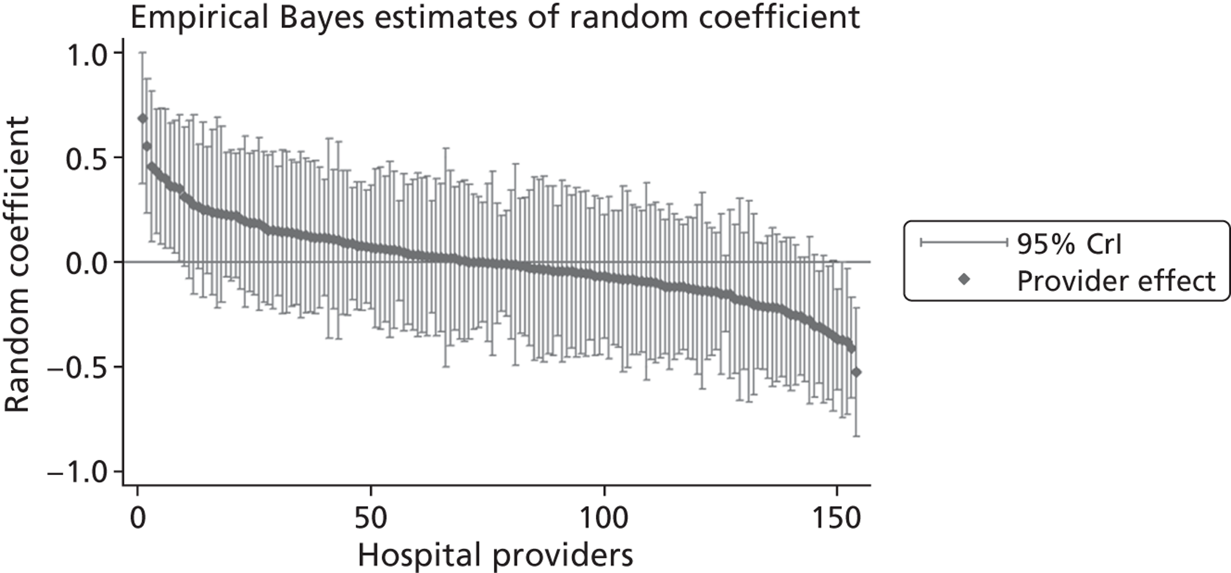
The graphical presentation of random coefficients as a caterpillar plot is informative in several ways. First, we find that variation among hospitals, as evidenced by the slope of the curve, is most pronounced on the mobility and usual activities dimensions. This is a reflection of the differences in estimated variance components that carry over to the EBE. Second, we find that only a small number of hospitals have a statistically significantly different treatment impact compared with the sample average, here standardised to zero. However, note that the CrIs are appropriate only for comparisons against zero, but are too wide for comparison of any two hospitals. 62 Third, CrIs on the mobility dimension are wider than on any other dimension of the EQ-5D. This reflects the lesser amount of information contained in the data, with only two mobility categories being reasonably well populated. The shortcoming of this type of analysis of hospital-specific random coefficients is it focuses on underlying health. Although it is possible to assess statistical significance, one cannot make statements about clinical or patient-perceived significance on the basis of the underlying health scale. To address this, we show hospital-specific probabilities of reporting a given post-treatment health status. In some cases, we find differences between hospitals to be quite remarkable. For example, the expected probabilities of reporting ‘no problems’ on usual activities, 6 months after surgery, ranges from 30% to 55.9%. In contrast, expected probabilities for the same category on the self-care dimension are significantly less dispersed and consistently above 80% for all hospitals.
Hospital performance on multiple EQ-5D dimensions
We explore the global agreement between estimates of hospital performance based on individual EQ-5D dimensions and the utility-weighted EQ-5D index values by calculating Spearman’s rank-order correlation coefficients (Spearman’s rho) and inspecting correlation patterns visually. Figure 8 shows plots of performance estimates on the underlying scale (for EQ-5D dimensions) compared with performance estimates on the EQ-5D utility scale. Consistent with discussion in The correlation between outcomes and costs and Risk-adjusted hospital performance on individual EQ-5D dimensions, zero indicates performance according to the benchmark expectation, negative values indicate worse than expected performance and positive values indicate better than expected performance.
FIGURE 8.
Hospital performance estimates on the EQ-5D dimensions and EQ-5D utility scores. (a) Mobility, Spearman’s rho = – 0.03; (b) self-care, Spearman’s rho = – 0.18*; (c) usual activities, Spearman’s rho = – 0.04; (d) pain/discomfort Spearman’s rho = – 0.48**; and (e) anxiety/depression Spearman’s rho = – 0.42***. *p < 0.05; **p < 0.01; ***p < 0.001.
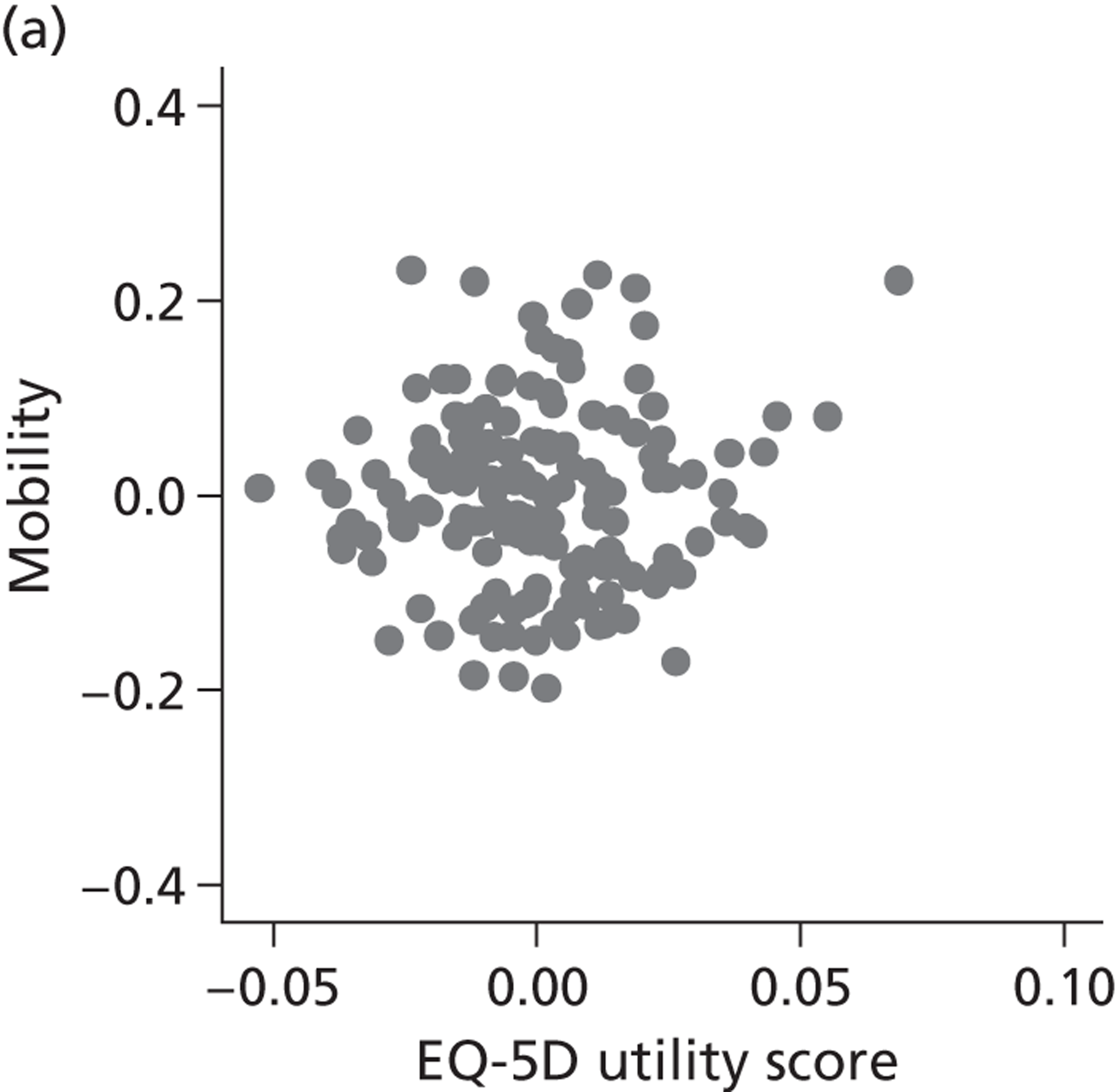
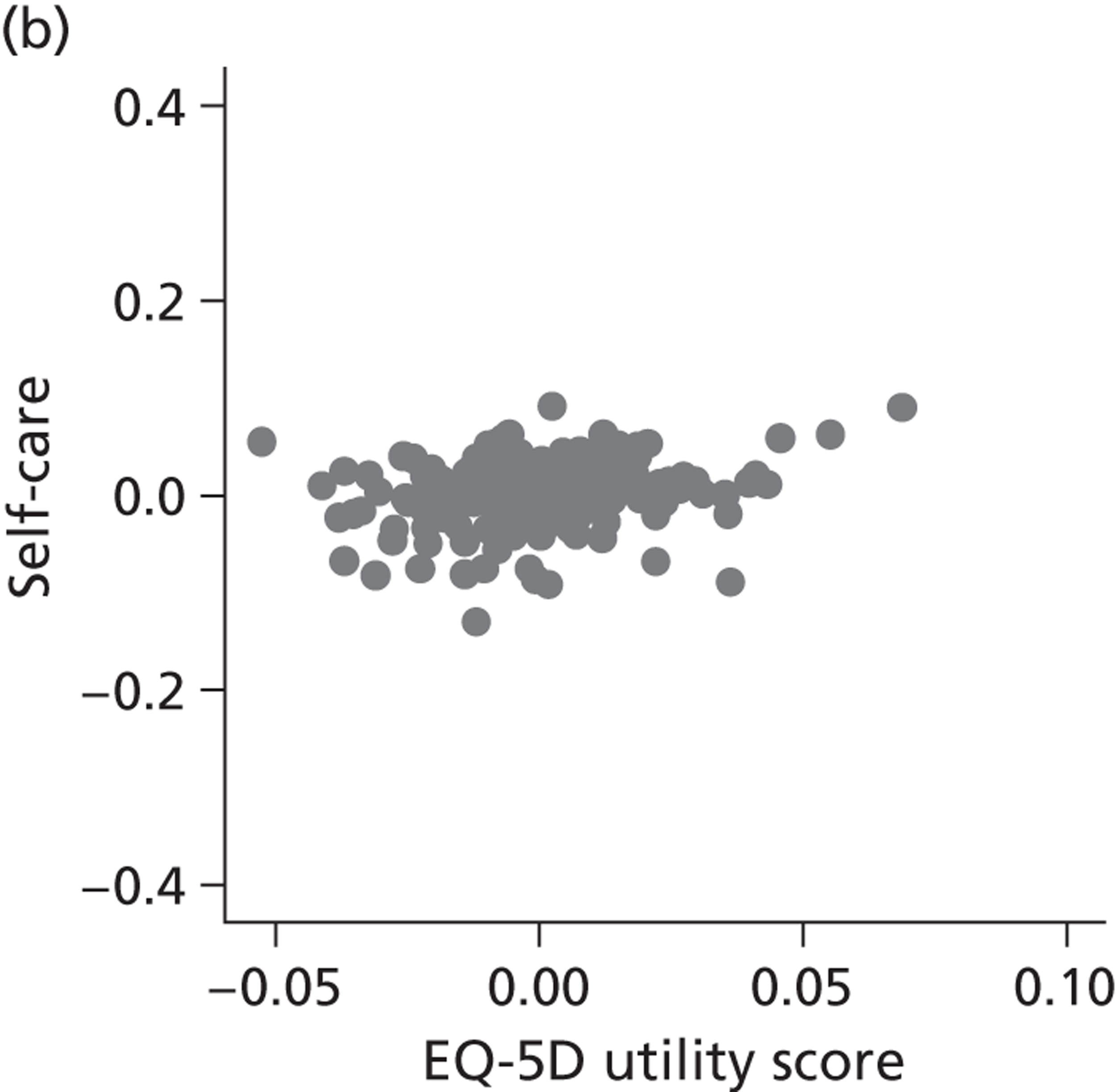
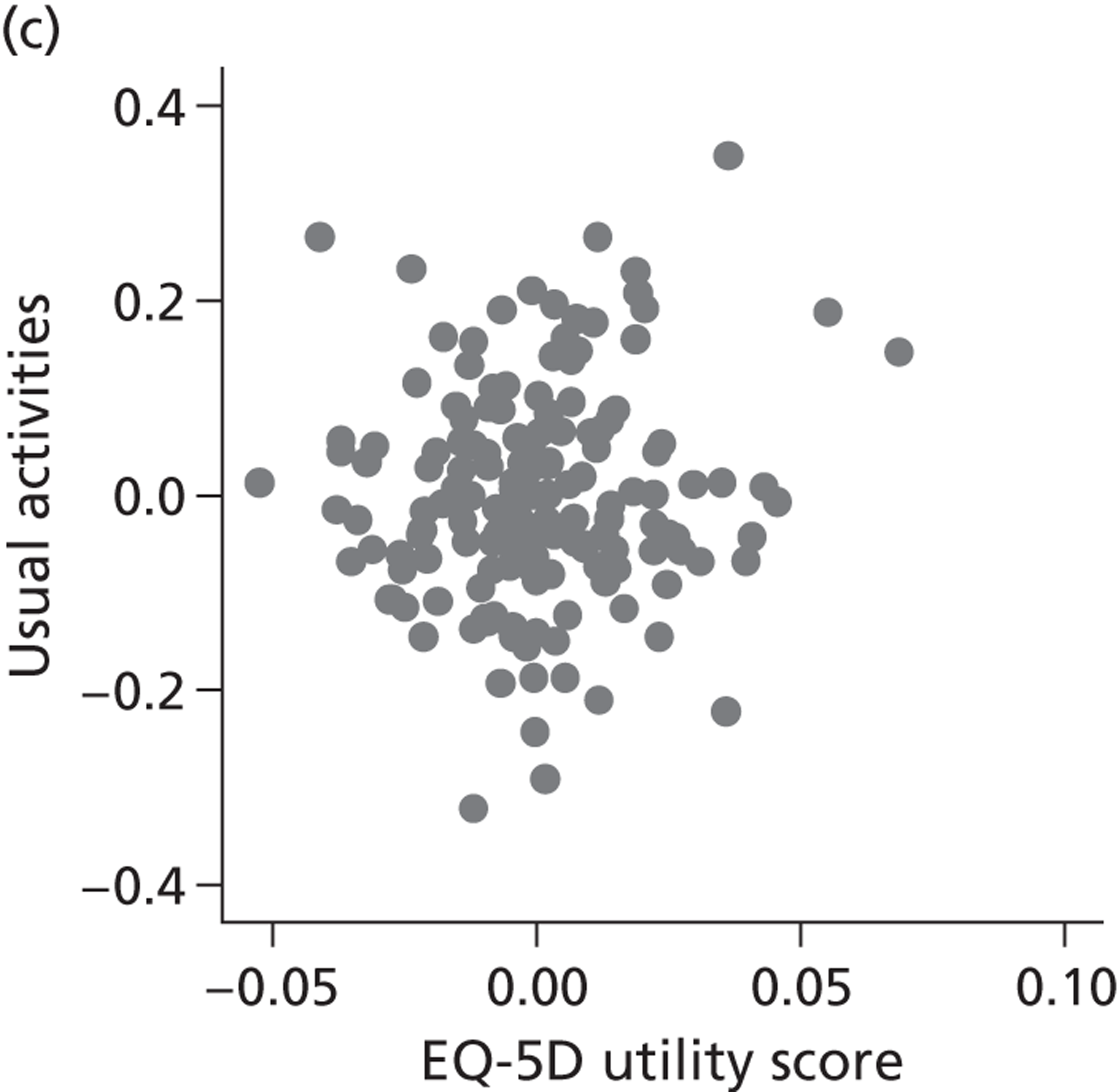
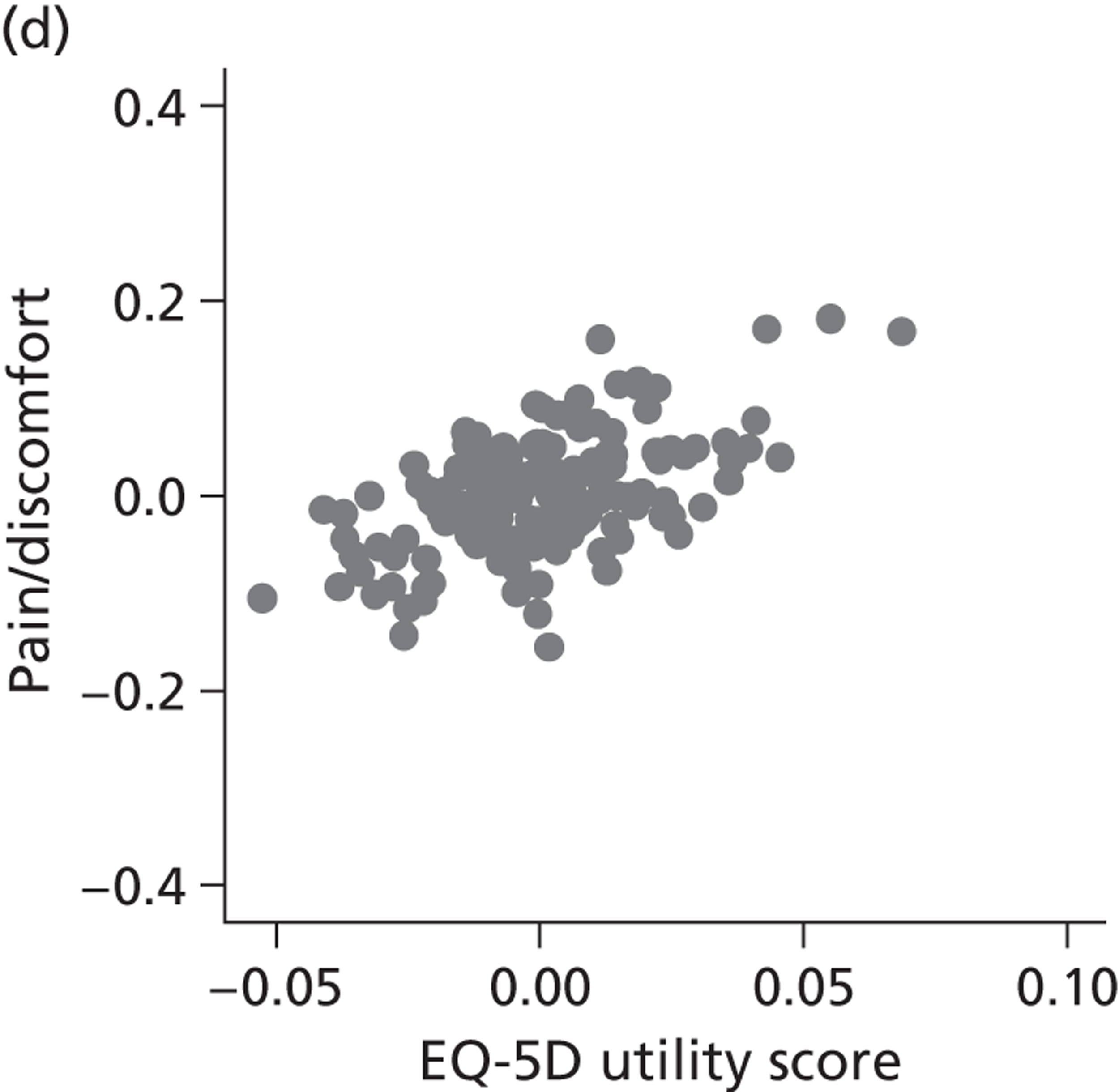
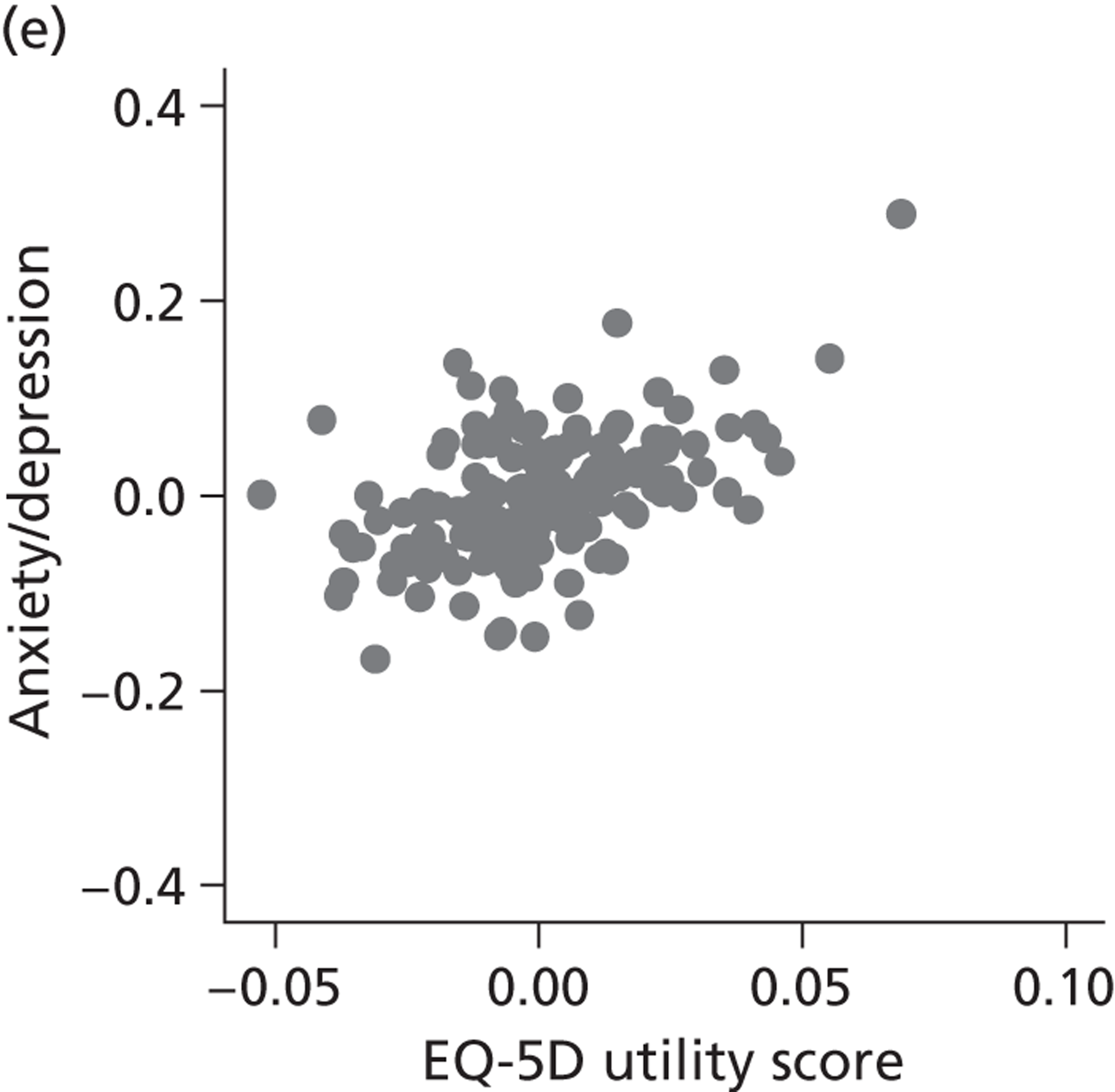
The highest rank correlation is observed between performance estimates on the pain/discomfort dimension and EQ-5D utility index (Spearman’s rho = 0.48), followed by the anxiety/depression dimension (Spearman’s rho = 0.42). The rank correlation for all other dimensions and the EQ-5D utility index is smaller (Spearman’s rho = < 0.2) and, indeed, not statistically significantly different from zero for the dimensions of mobility and usual activities.
The relationship between cost of treatment and outcomes
Methodology and statistical approach
To assess the relationship between resource use and health outcomes, we use random-effects multilevel models to distinguish between systematic hospital-specific effects, the impact of differing patient case mix and random variation. The equations are estimated in a seemingly unrelated regression (SUR) framework to allow for correlation between resource use and health outcomes due to common omitted variables. 63 The EBE of the hospital-specific effects are the main focus of the analysis.
Data are analysed at patient level with patients i = 1, . . . , N j clustered within hospitals j = 1, . . . , J with achievements C ij and H ij 1 associated with the health production and the cost functions k ε [c, h]. We assume a linear additive relationship between these achievements and a hospital-specific intercept, γ j,k , a constant term, α k , a set of patient-level risk-adjustment variables, X ij,k and a set of hospital-level explanatory variables, Z j,k , all of which may differ across equations. The model can be written as:
where β c , β h , θ c and θ h are vectors of parameters to be estimated and which relate patient and hospital characteristics to postoperative health status and costs.
By estimating the model as a system of equations in a SUR framework rather than each equation in isolation, it is possible to measure directly the covariance and correlation in the error terms at both the patient and the hospital level. The random effects at patient level are assumed to be a draw from a bivariate normal distribution such that
and at hospital level
with ρ 1 ε[– 1,1] being a measure of correlation at patient level and ρ 2 ε[– 1,1] measuring correlation at hospital level. Correlation between error terms, which would occur with ρ 1 ≠ 0 and/or ρ 2 ≠ 0, indicates common omitted variables across cost and health production equations at the relevant level. For example, if there were an omitted patient characteristic that made healthy outcomes less likely while at the same time increasing costs, we would expect ρ 1 to be negative.
The correlation coefficient, ρ 2, is of greater interest and reflects a population-averaged relationship between the estimates of γ ^ j , c and γ ^ j , h . These capture the hospital-specific effects after allowing for the hospital’s patient case mix and relevant production constraints, and form our estimate of the hospital-specific deviation from the benchmark, i.e. ( E j , k − E ¯ k ) . Accordingly, γ ^ j , c above (or below) zero indicate that, all other things being equal, the hospital has above (or below) average costs, increasing in the magnitude of the coefficient. Similarly, values of γ ^ j , h above (or below) zero indicate that, all other things being equal, the hospital has above (or below) average health outcomes. A positive correlation coefficient, ρ 2, would indicate that higher costs are generally associated with higher health gains (and vice versa), i.e. a trade-off between efforts to contain costs and provide high-quality care. A negative correlation would indicate that efforts to contain costs are associated with efforts to provide high-quality care. A zero correlation would indicate no relationship.
All models are estimated in Multilevel modelling for Windows computer package (MlwiN; Centre for Multilevel Modelling, Bristol, UK) using iterative generalised least squares (IGLS), equivalent to full maximum likelihood. Alternatively, we could estimate this model using GLLAMM for Stata 12; however, MLwiN is computationally more efficient. All data management and visualisations are done in GLLAMM for Stata 12. The link between GLLAMM for Stata 12 and MLwiN is provided by the user-written program runmlwin (Centre for Multilevel Modelling, University of Bristol, UK),64 the Stata module for fitting multilevel models in the MLwiN software package. 64 We obtain EBE of γ ^ j , c and γ ^ j , h with accompanying 95% CrIs in postestimation, with the unknown population parameters substituted by estimated variance components and parameters. Hospitals are considered to be situated within one quadrant of the performance space illustrated in Figure 1 if both CrIs do not contain zero.
Descriptive statistics
Patient level
Table 6 reports descriptive statistics for patients undergoing each of the four procedures. Our overall sample consists of 48,008 patients and knee replacement is the most frequently observed procedure and varicose vein surgery is the least frequently observed.
| Variable | Description | Hip replacement | Knee replacement | Groin hernia repair | Varicose vein surgery | ||||
|---|---|---|---|---|---|---|---|---|---|
| Mean | SD | Mean | SD | Mean | SD | Mean | SD | ||
| Resource use | |||||||||
| costs | Cost of care in £000, adjusted for MFF | 6.22 | 1.93 | 6.19 | 2.06 | 1.44 | 0.65 | 1.21 | 0.61 |
| los | Length of hospital stay (days) | 5.85 | 4.05 | 5.74 | 3.54 | 0.42 | 0.89 | 0.14 | 0.47 |
| Post-treatment health | |||||||||
| post_cond | Post-operative condition-specific score | 38.08 | 9.41 | 33.48 | 10.12 | – | – | 89.38 | 9.53 |
| post_EQ5D | Post-operative EQ-5D index score | 0.76 | 0.25 | 0.70 | 0.27 | 0.88 | 0.18 | 0.87 | 0.19 |
| post_EQVAS | Post-operative EQ-VAS score | 75.37 | 18.14 | 71.56 | 18.69 | 79.73 | 15.67 | 80.25 | 15.83 |
| Explanatory factors | |||||||||
| pre_cond | Pre-operative condition-specific score | 18.34 | 8.38 | 18.81 | 7.68 | 0.00 | 0.00 | 81.38 | 9.85 |
| pre_EQ5D | Pre-operative EQ-5D index score | 0.36 | 0.32 | 0.40 | 0.31 | 0.79 | 0.19 | 0.78 | 0.20 |
| pre_EQVAS | Pre-operative EQ-VAS score | 66.16 | 20.95 | 68.46 | 19.21 | 80.74 | 14.35 | 80.45 | 15.24 |
| age | Age of patient (years) | 67.38 | 10.85 | 68.79 | 9.17 | 61.23 | 14.41 | 52.00 | 13.92 |
| male | Indicator for male gender | 0.43 | 0.49 | 0.45 | 0.50 | 0.93 | 0.25 | 0.35 | 0.48 |
| wcharlson | Weighted Charlson index | 0.30 | 0.64 | 0.36 | 0.67 | 0.17 | 0.48 | 0.08 | 0.30 |
| add_diagnoses | Number of additional diagnoses | 1.90 | 1.79 | 2.00 | 1.84 | 0.90 | 1.30 | 0.44 | 0.90 |
| revision | Indicator for revision surgery | 0.07 | 0.26 | 0.05 | 0.21 | – | – | – | – |
| deprivation | IMD – income domain58 | 0.12 | 0.09 | 0.13 | 0.10 | 0.13 | 0.10 | 0.14 | 0.11 |
| multiepi | Indicator for multiple consultants during hospital stay | 0.01 | 0.12 | 0.01 | 0.10 | 0.00 | 0.07 | 0.00 | 0.05 |
| HRG1 | Indicator for most common HRG | 0.82 | 0.38 | 0.85 | 0.35 | 0.83 | 0.38 | 0.76 | 0.43 |
| HRG2 | Indicator for second most common HRG | 0.04 | 0.21 | 0.05 | 0.22 | 0.14 | 0.34 | 0.11 | 0.31 |
| HRG3 | Indicator for third most common HRG | 0.04 | 0.18 | 0.05 | 0.21 | 0.02 | 0.13 | 0.06 | 0.24 |
| HRG4 | Indicator for fourth most common HRG | 0.04 | 0.18 | 0.03 | 0.17 | 0.00 | 0.06 | 0.05 | 0.21 |
| HRG5 | Indicator for fifth most common HRG | 0.02 | 0.15 | 0.00 | 0.06 | 0.00 | 0.06 | 0.01 | 0.10 |
| HRGother | Indicator for any other HRG | 0.04 | 0.19 | 0.01 | 0.11 | 0.01 | 0.11 | 0.02 | 0.12 |
| Number of observations | |||||||||
| n | Total number of patients | 16,403 | 17,444 | 10,389 | 3772 | ||||
| J | Hospitals | 142 | 143 | 146 | 130 | ||||
Mean costs are similar for hip and knee replacements (around £6200) and considerably lower for groin hernia repair and varicose vein surgery (< £1500). Average LoS is also much lower for the last two procedures, with such patients rarely requiring an overnight stay. As LoS is measured as full inpatient days, we observe only very limited variation in this measure of resource use for groin hernia and varicose vein surgery.
The EQ-5D scores suggest that average post-treatment health status is lower following hip (0.76) and knee (0.70) replacement than it is for hernia repair (0.88) and varicose vein surgery (0.87). But for the last two procedures, pretreatment scores are also quite high (> 0.77). In contrast, pretreatment scores are relatively low for patients about to undergo hip (0.36) and knee (0.40) replacement. The change in mean health status as a result of surgery is, therefore, quite considerably larger for hip and knee replacement than it is for hernia repair or varicose vein surgery. The condition-specific measures, where available, tell a similar story.
Summary statistics for the variables used as risk adjusters reveal different patterns in the age and gender profiles of the patients undergoing each procedure. They also differ in terms of the complexity measures, those having hip or knee replacement having higher weighted Charlson scores and more additional diagnoses than the other patients. There are no obvious differences across procedures in terms of the socioeconomic deprivation profile of the neighbourhood in which patients reside.
The HRG variables are specific to each procedure. Over 75% of patients undergoing each type of procedure are allocated a single HRG, which forms the reference category in each regression.
Table 7 shows the variation in mean PROM scores (pretreatment, post treatment and the difference between the two), costs, LoS and number of patients treated among hospitals for each of the four conditions. Patients are clustered in 130 to 146 hospitals and the average number of patients treated by each hospital ranges from 29 (varicose vein surgery) to 122 (knee replacement surgery). Note that the presented values describe the characteristics of the distribution of hospital-average scores rather than the distribution of patient characteristics.
| Mean of sample values | SD | Minimum of sample values | 25th pct | Median | 75th pct | Maximum of sample values | |
|---|---|---|---|---|---|---|---|
| Hip replacement (142 hospitals) | |||||||
| Number of patients treated | 115.51 | 82.81 | 9 | 55 | 97 | 161 | 462 |
| Pre-treatment EQ-5D utility | 0.35 | 0.06 | 0.10 | 0.30 | 0.35 | 0.39 | 0.55 |
| Post-treatment EQ-5D utility | 0.75 | 0.06 | 0.55 | 0.72 | 0.76 | 0.80 | 0.89 |
| Change in EQ-5D utility | 0.41 | 0.05 | 0.19 | 0.38 | 0.41 | 0.44 | 0.54 |
| Pre-treatment EQ-VAS score | 65.52 | 3.36 | 55.72 | 63.68 | 65.71 | 67.50 | 73.13 |
| Post-treatment EQ-VAS score | 74.74 | 3.80 | 54.50 | 73.20 | 75.44 | 77.10 | 82.33 |
| Change in EQ-VAS score | 9.22 | 3.90 | – 7.90 | 7.13 | 9.42 | 11.65 | 22.27 |
| Pre-treatment OHS | 18.08 | 1.70 | 13.50 | 16.87 | 17.91 | 19.22 | 22.63 |
| Post-treatment OHS | 37.75 | 2.20 | 29.89 | 36.64 | 38.08 | 39.23 | 42.11 |
| Change in OHS | 19.68 | 1.79 | 12.17 | 18.78 | 19.76 | 20.90 | 23.94 |
| Costs adjusted for MFF (in £000) | 6.29 | 1.71 | 1.63 | 5.22 | 6.01 | 7.02 | 14.75 |
| LoS | 6.08 | 1.25 | 3.90 | 5.33 | 5.96 | 6.57 | 13.50 |
| Knee replacement (143 hospitals) | |||||||
| Number of patients treated | 121.99 | 84.89 | 1 | 61 | 99 | 171 | 459 |
| Pre-treatment EQ-5D utility | 0.39 | 0.07 | 0.03 | 0.36 | 0.40 | 0.43 | 0.55 |
| Post-treatment EQ-5D utility | 0.69 | 0.05 | 0.49 | 0.66 | 0.69 | 0.73 | 0.85 |
| Change in EQ-5D utility | 0.30 | 0.07 | 0.11 | 0.26 | 0.30 | 0.32 | 0.82 |
| Pre-treatment EQ-VAS score | 67.65 | 4.59 | 40.00 | 65.94 | 68.11 | 70.17 | 77.59 |
| Post-treatment EQ-VAS score | 71.30 | 3.51 | 59.85 | 69.42 | 71.61 | 73.91 | 80.19 |
| Change in EQ-VAS score | 3.65 | 3.39 | – 1.69 | 1.69 | 3.17 | 5.04 | 25.83 |
| Pre-treatment OKS | 18.57 | 1.92 | 11.00 | 17.55 | 18.62 | 19.77 | 22.67 |
| Post-treatment OKS | 33.34 | 2.29 | 26.47 | 32.11 | 33.26 | 34.94 | 41.00 |
| Change in OKS | 14.77 | 2.05 | 10.04 | 13.62 | 14.64 | 15.56 | 29.00 |
| Costs adjusted for MFF (in £000) | 6.31 | 1.84 | 1.54 | 5.32 | 5.98 | 7.01 | 16.14 |
| LoS | 5.90 | 1.11 | 3.85 | 5.21 | 5.74 | 6.37 | 12.67 |
| Groin hernia repair (146 hospitals) | |||||||
| Number of patients treated | 71.16 | 53.29 | 1 | 37 | 61 | 89 | 365 |
| Pre-treatment EQ-5D utility | 0.79 | 0.04 | 0.60 | 0.78 | 0.79 | 0.82 | 0.94 |
| Post-treatment EQ-5D utility | 0.88 | 0.03 | 0.77 | 0.86 | 0.88 | 0.90 | 1.00 |
| Change in EQ-5D utility | 0.09 | 0.04 | – 0.08 | 0.06 | 0.09 | 0.10 | 0.31 |
| Pre-treatment EQ-VAS score | 80.63 | 3.11 | 67.00 | 79.12 | 80.68 | 82.40 | 100.00 |
| Post-treatment EQ-VAS score | 79.62 | 2.67 | 71.00 | 77.99 | 79.69 | 81.31 | 87.33 |
| Change in EQ-VAS score | – 1.01 | 2.39 | – 15.00 | – 2.11 | – 1.01 | 0.10 | 6.56 |
| Costs adjusted for MFF (in £000) | 1.52 | 0.55 | 0.53 | 1.23 | 1.49 | 1.77 | 5.69 |
| LoS | 0.44 | 0.25 | 0.00 | 0.27 | 0.38 | 0.57 | 1.37 |
| Varicose vein surgery (130 hospitals) | |||||||
| Number of patients treated | 29.02 | 32.51 | 1 | 8 | 23 | 40 | 190 |
| Pre-treatment EQ-5D utility | 0.77 | 0.07 | 0.46 | 0.74 | 0.78 | 0.81 | 1.00 |
| Post-treatment EQ-5D utility | 0.87 | 0.09 | 0.12 | 0.84 | 0.88 | 0.91 | 1.00 |
| Change in EQ-5D utility | 0.10 | 0.11 | – 0.88 | 0.07 | 0.10 | 0.13 | 0.44 |
| Pre-treatment EQ-VAS score | 80.36 | 5.89 | 50.00 | 77.00 | 80.04 | 83.95 | 95.00 |
| Post-treatment EQ-VAS score | 80.24 | 5.57 | 60.00 | 77.50 | 81.22 | 83.83 | 91.30 |
| Change in EQ-VAS score | – 0.12 | 4.58 | – 15.67 | – 2.56 | – 0.36 | 2.50 | 20.00 |
| Pre-treatment AVVS | 80.76 | 4.04 | 66.13 | 78.95 | 81.33 | 83.38 | 90.39 |
| Post-treatment AVVS | 89.33 | 3.85 | 66.63 | 87.45 | 89.64 | 91.47 | 99.33 |
| Change in AVVS | 8.56 | 3.35 | – 5.82 | 6.57 | 8.82 | 10.66 | 19.93 |
| Costs adjusted for MFF (in £000) | 1.22 | 0.48 | 0.12 | 0.86 | 1.15 | 1.57 | 2.53 |
| LoS | 0.18 | 0.23 | 0.00 | 0.00 | 0.11 | 0.25 | 1.29 |
As with the patient-level descriptive statistics, there are noticeable differences between mean EQ-5D utility scores across hospitals and conditions, for both pre- and post-treatment scores. This is illustrated in the box plots in Figures 9–11 . The shaded boxes and the ‘whiskers’ are all approximately the same size for all conditions for pretreatment means and post-treatment means, both within and across procedures. The observed mean pre- and post-treatment EQ-5D utility scores ( Figure 9 ) are lower for hip and knee replacement surgery than for varicose vein surgery or groin hernia repair. However, despite the difference in the general location on the EQ-5D utilities, the variation in means across hospitals is broadly similar, whether measured by the standard deviation or the interquartile range (IQR), i.e. the difference between the 25th and 75th percentiles of the distribution. In other words, the three box plots (excluding the outliers) are generally distinguishable only by their location, not their size.
FIGURE 9.
Distribution of average EQ-5D utility scores before and after treatment across hospitals.
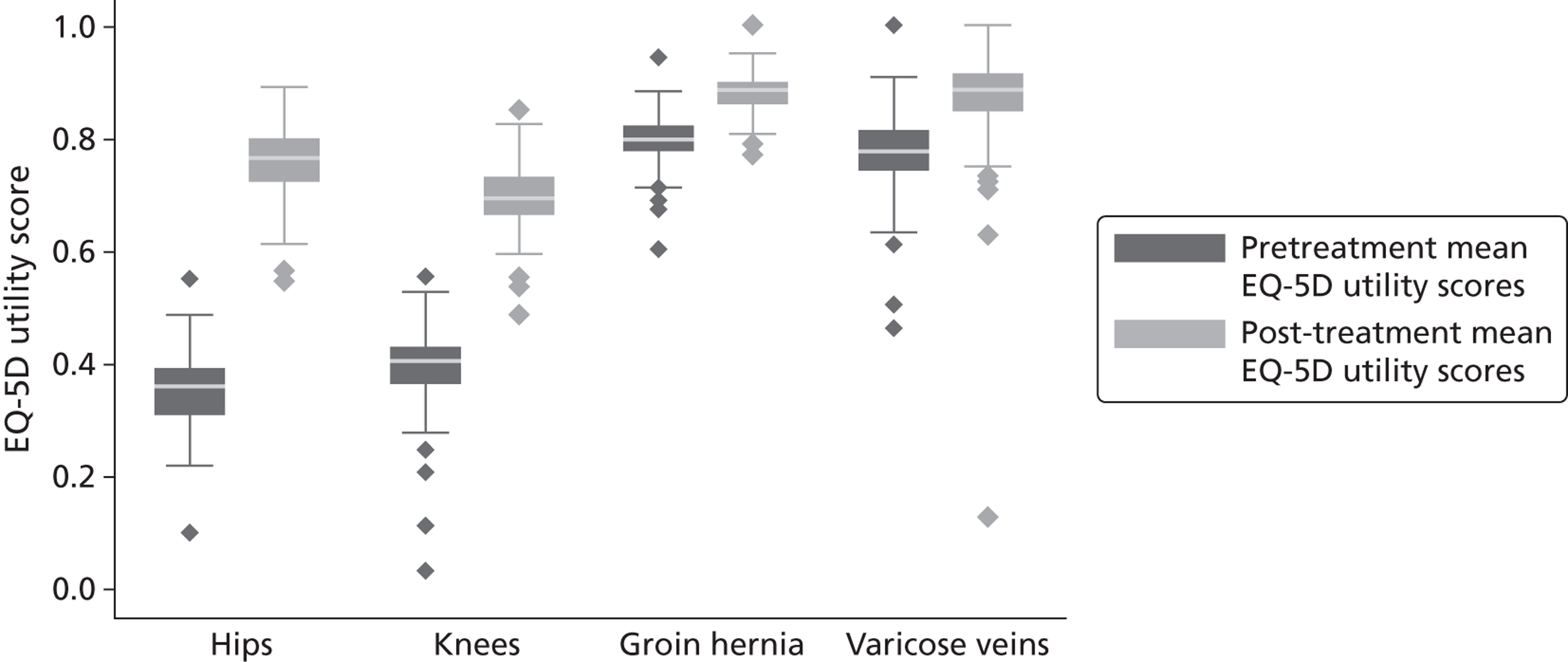
FIGURE 10.
Distribution of average EQ-VAS scores before and after treatment across hospitals.
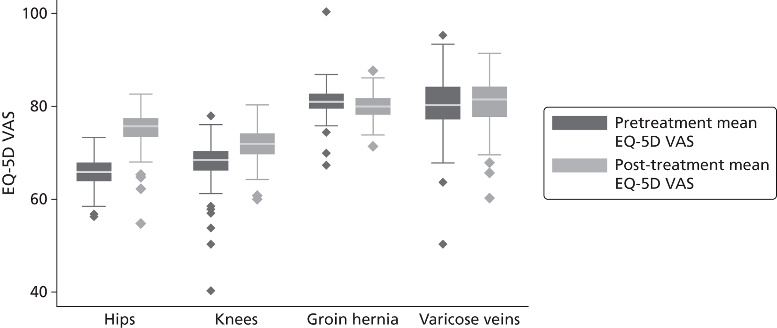
FIGURE 11.
Distribution of average condition-specific instrument scores before and after treatment across hospitals.
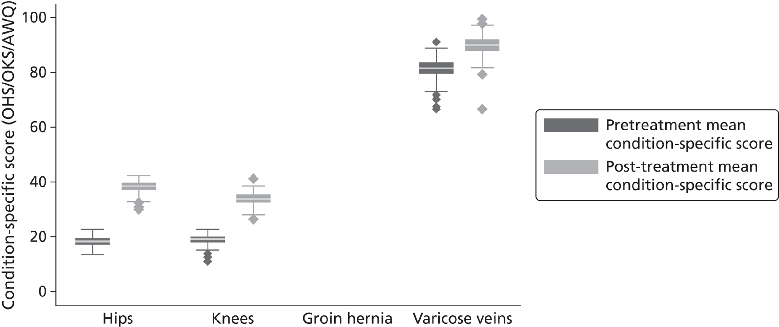
The EQ-5D utility scores ( Figure 9 ) and condition-specific measures (where applicable – Figure 11 ) all suggest improvements in health status, as indicated by the upward shift in the location of the pre- and post-treatment box plots. In contrast, the EQ-VAS ( Figure 10 ) shows little change in the pre- and post-treatment distributions for knees, a negative change for groin hernia and no change for varicose veins.
While the main bodies of the distributions of pre- and post-treatment EQ-5D utility scores across conditions show little difference, there is a clear change with regards to the distribution of outliers. For hip replacement, knee replacement and especially groin hernia repair, the dispersion of outliers (shown as above or below the ‘whiskers’) decreases noticeably after treatment. The exception is varicose vein surgery, where the dispersion of outliers post treatment is higher than pretreatment and may have been even higher if utility scores were not bound at the upper limit of one (‘full health’). Such patterns are not apparent when the EQ-VAS is considered.
Figure 12 shows the distribution of average resource use across hospitals, measured using cost of treatment and LoS. There are three points of note. First, the location of the cost and LoS distributions is similar for hip and knee replacement, but the LoS distribution is lower than the cost distribution for groin hernia and varicose veins. This is because the groin hernia and varicose veins tend to be treated on a day-case basis. Second, there is a wider distribution for costs than LoS, which reflects the fewer and lower values of LoS compared with cost of treatment. Third, for hip replacement and knee replacement, there are a handful of hospitals with extreme costs of treatment or LoS. There are just a couple of hospitals at the upper extremes for groin hernia and varicose veins.
FIGURE 12.
Distribution of average, unadjusted resource use by hospital.
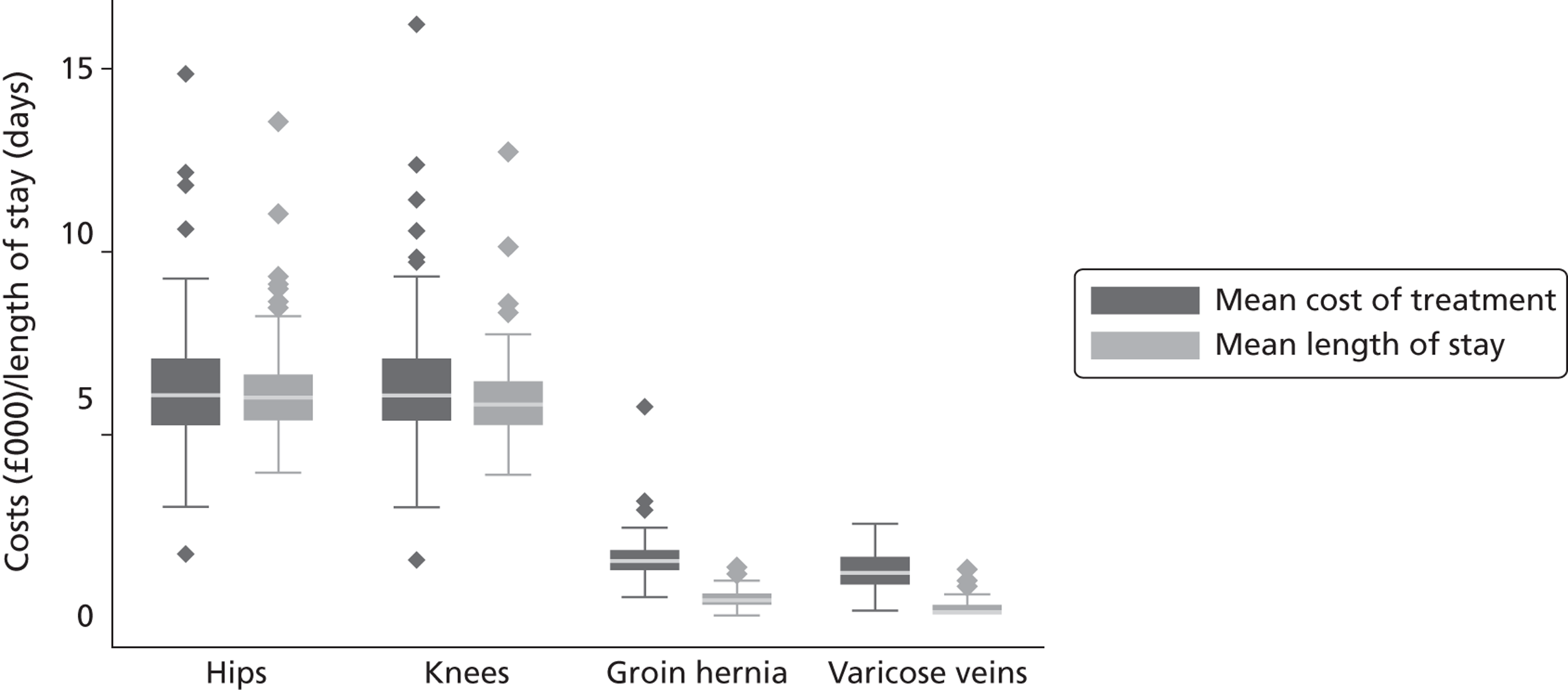
Unadjusted outcome/cost ratios
Figures 13–16 present unadjusted outcome/cost ratios for the four conditions. The IQRs reflect the variability in outcome/cost ratios within each hospital. We do not present graphs with respect to LoS because many patients, especially those undergoing groin hernia repair or varicose vein surgery, do not stay overnight and, hence, the ratio of outcomes to LoS is undefined.
FIGURE 13.
Outcome/cost ratios by hospital – hip replacement. (a) EQ-5D utility index; (b) EQ-VAS; and (c) OHS.
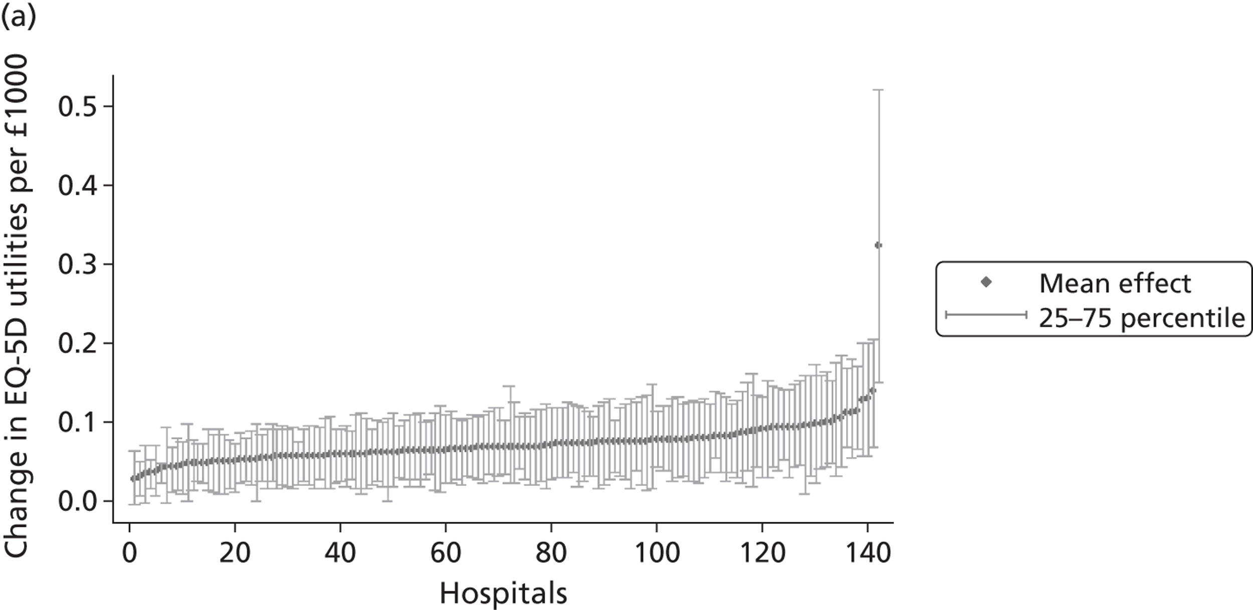
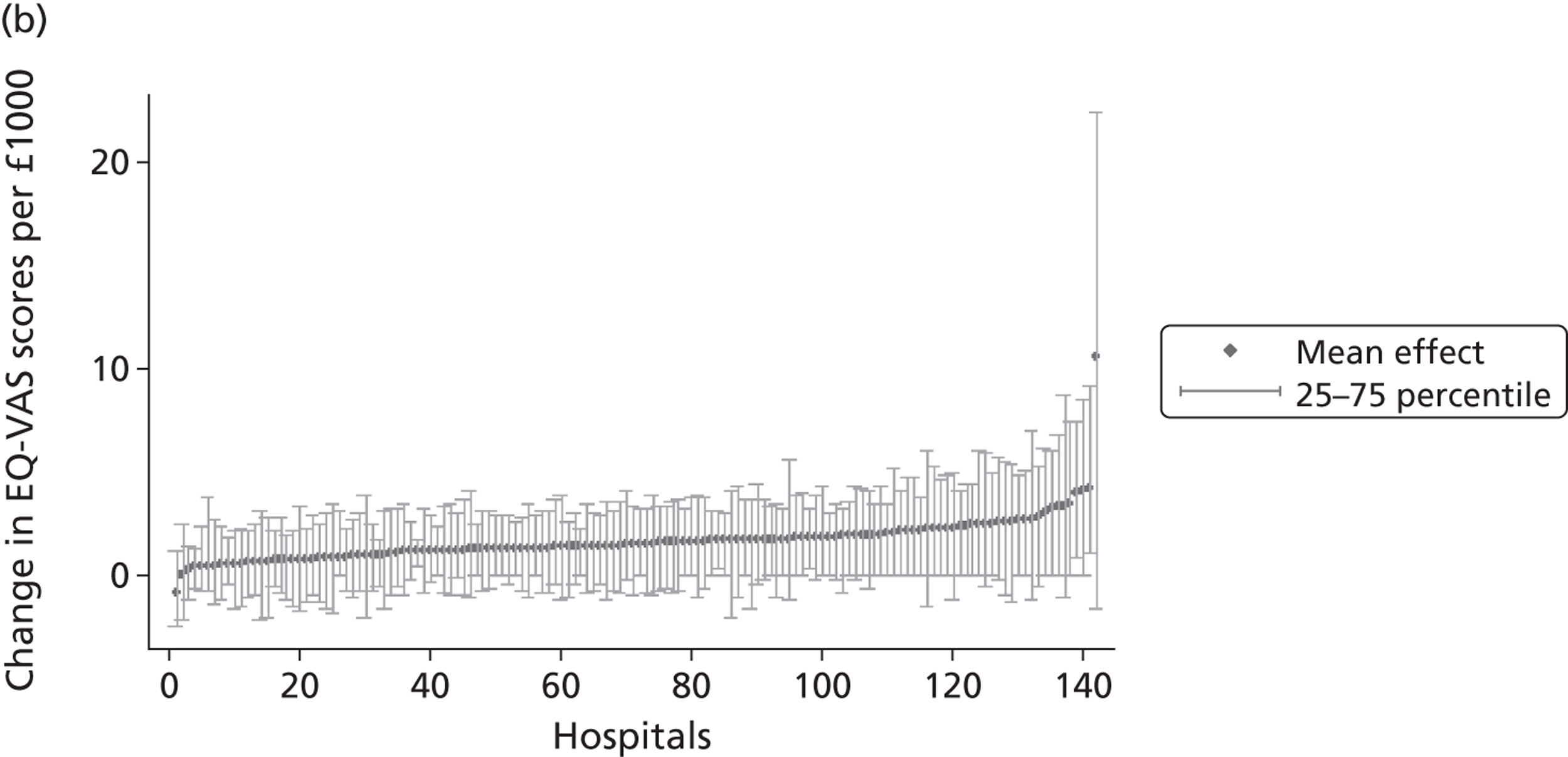
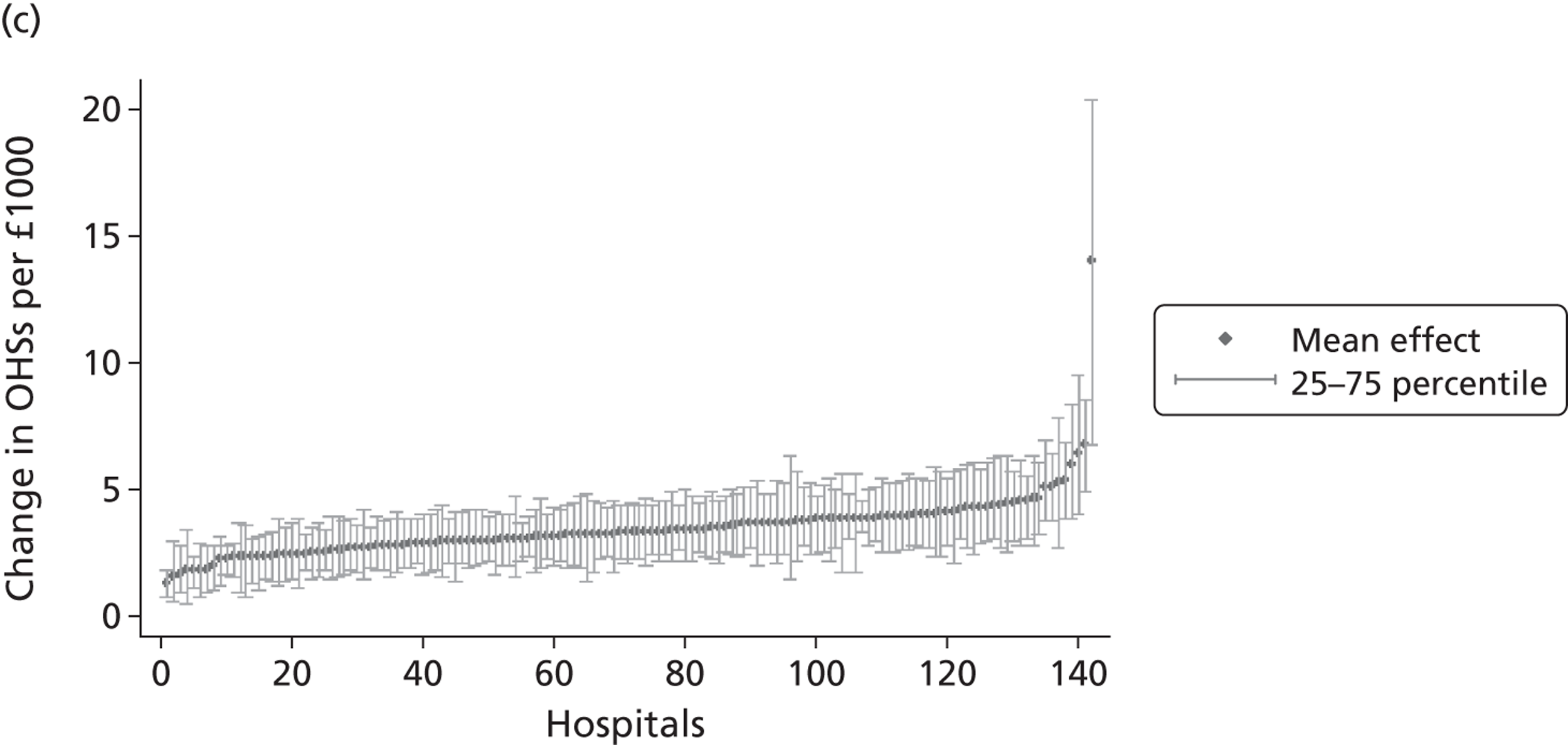
FIGURE 14.
Outcome/cost ratios by hospital – knee replacement. (a) EQ-5D utility index; (b) EQ-VAS; and (c) OKS.
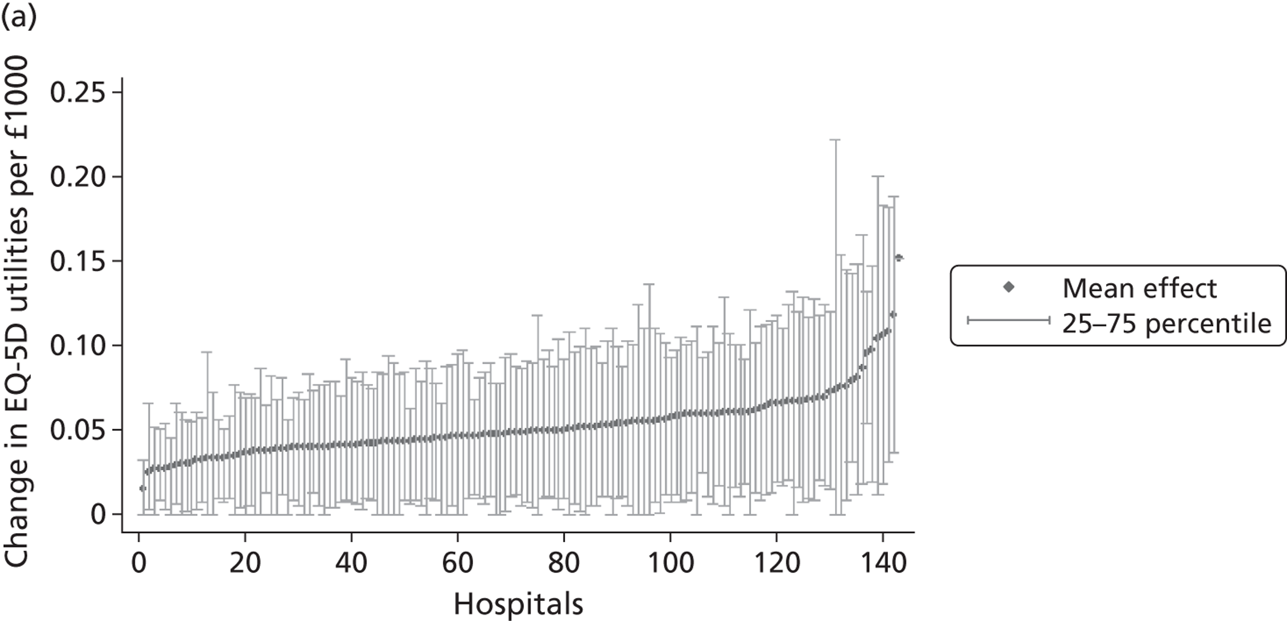
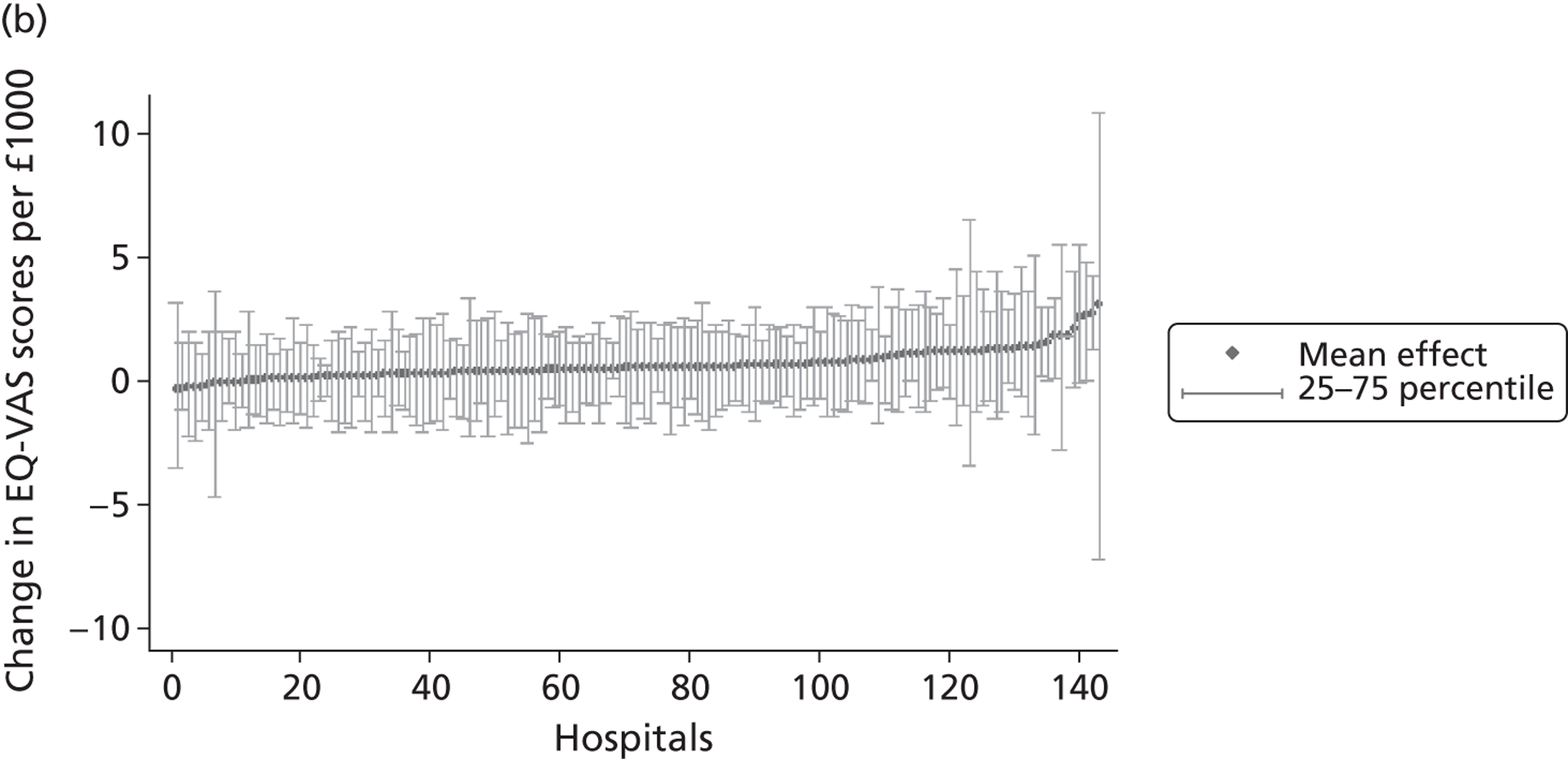
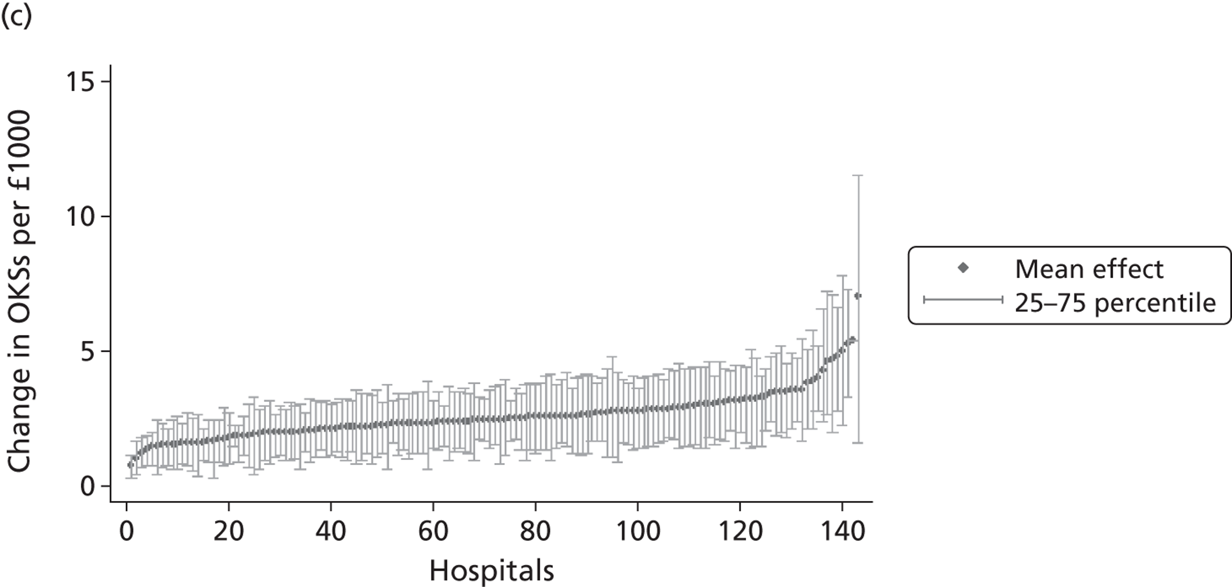
FIGURE 15.
Outcome/cost ratios by hospital – groin hernia repair. (a) EQ-5D utility index; and (b) EQ-VAS.
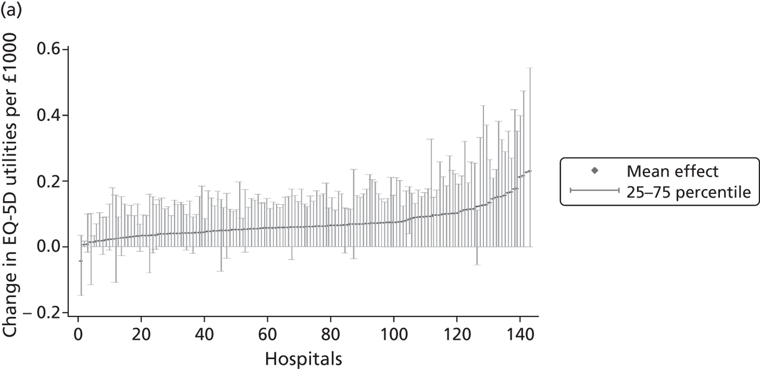
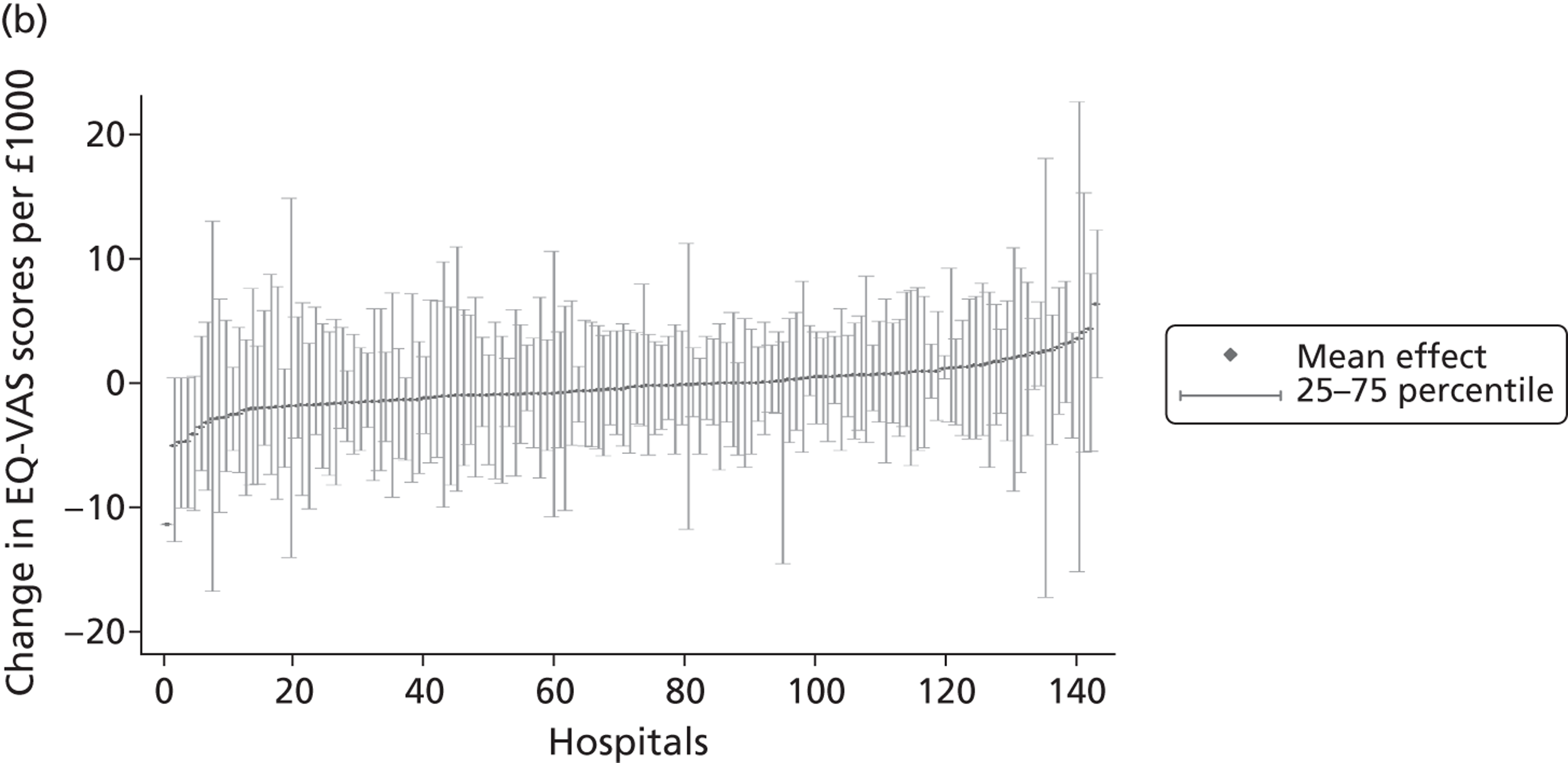
FIGURE 16.
Outcome/cost ratios by hospital – varicose vein surgery. (a) EQ-5D utility index; (b) EQ-VAS; and (c) AVVQ score.
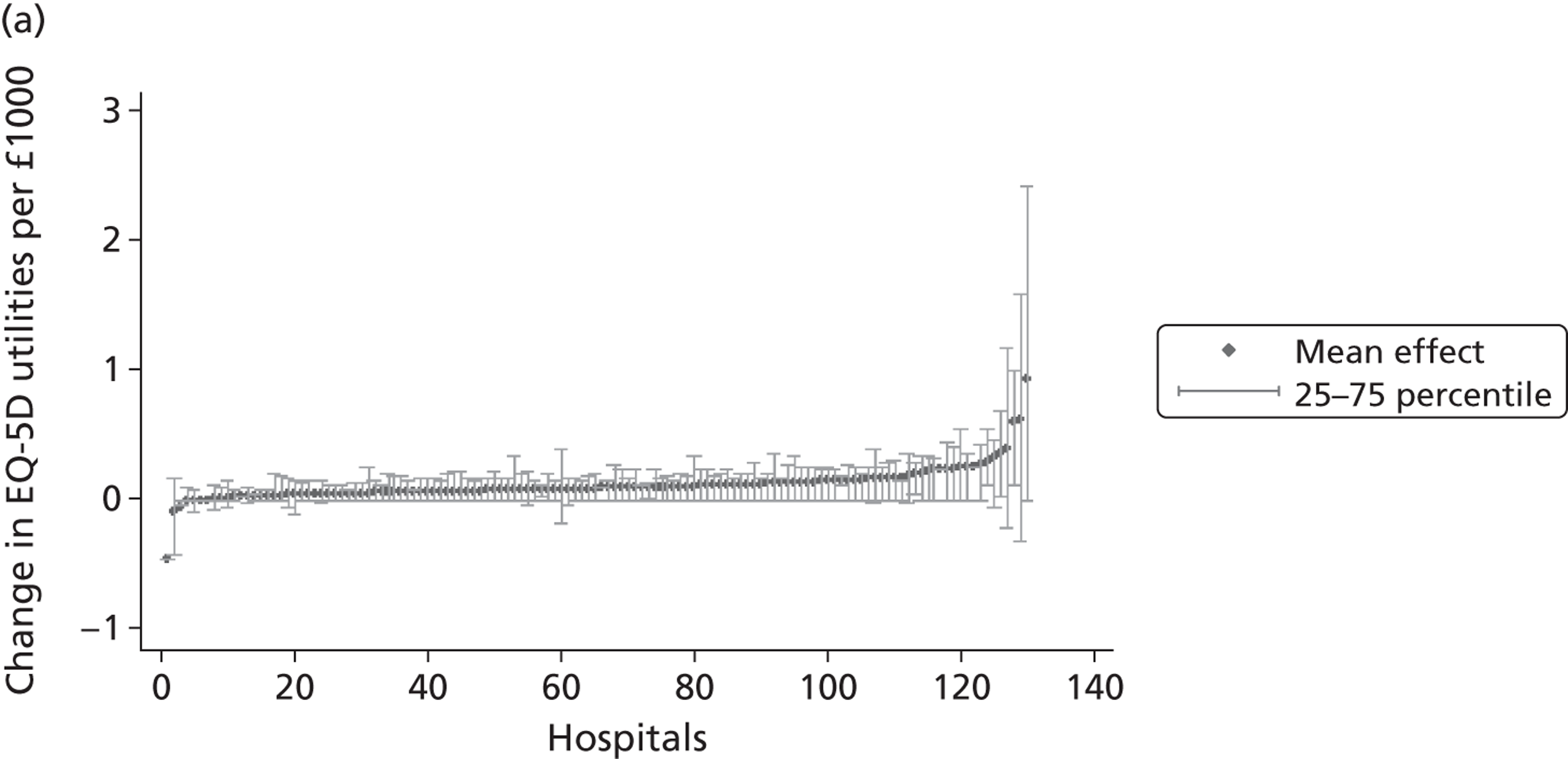
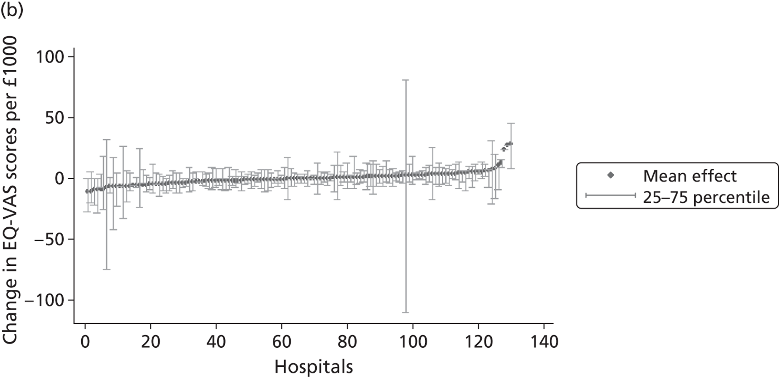
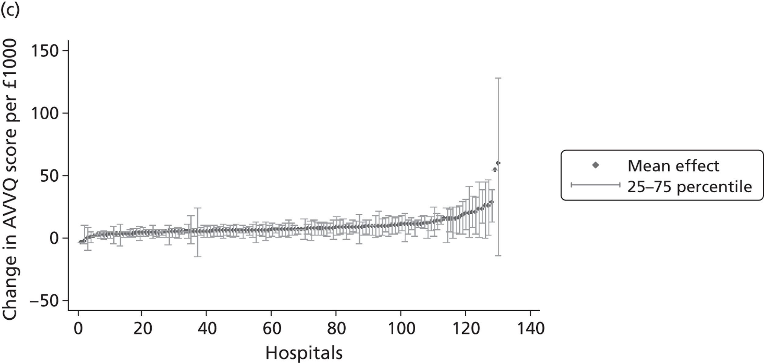
Average costs differ substantially across hospitals. This leads to different amounts of health outcome generated per unit of cost across hospitals. Those hospitals that generate more health outcome per unit of cost also have a larger IQR, i.e. there is more variability within these hospitals. This finding is independent of the PROM used.
Outcome/cost ratios can be compared across procedures when outcomes are measured by the EQ-5D utility index or EQ-VAS. The highest average level of utility gain per unit of cost is observed for varicose vein surgery (0.113 per £1000), where a small gain in health outcome is produced at very low costs. The smallest average utility gain per unit of cost is observed for knee replacement surgery with 0.053 units of health gain per £1000. Here, the larger utility gains are offset by proportionally higher costs.
As expected from the box plots on pre- and post-treatment operative EQ-VAS scores, we find that many hospitals have, on average, negative EQ-VAS health outcomes that translate into negative outcome/cost ratios. This is especially pronounced for varicose vein surgery and groin hernia repair, where more than half of the hospitals achieve negative outcome/cost ratios. This is counter to what we observe for EQ-5D outcome/cost ratios. Thus, the general interpretation of the unadjusted outcome/cost ratios is sensitive to the choice of generic PROM used.
Missing data
Tables 8–11 present a comparison of patient characteristics and resource use for patients included in our analytical sample with those excluded. Patients are only included if they have provided health status measures both pre- and post-treatment on all PROMs. For the purpose of the analysis, we pool observations for patients who (1) did not participate, (2) participated in the initial survey but were lost to follow-up or (3) participated but provided incomplete data. The groups are compared by means of two-sided t-tests with adjustment for unequal variances. Additionally, we also ran logistic regressions on the probability of being included in our estimation sample, conditional on the observed patient characteristics and the incurred resource use.
| Variablea | Excluded (SD) | Included (SD) | p-valueb | Odds ratio (z-value) |
|---|---|---|---|---|
| age | 68.33 (11.84) | 67.38 (10.85) | 0.000 | 1.00 (0.44) |
| male | 0.40 (0.49) | 0.43 (0.49) | 0.000 | 1.07 (3.32) |
| wcharlson | 0.35 (0.72) | 0.30 (0.64) | 0.000 | 0.94 (3.34) |
| add_diagnoses | 2.09 (1.97) | 1.90 (1.79) | 0.000 | 0.98 (1.83) |
| revision | 0.13 (0.33) | 0.07 (0.26) | 0.000 | 0.55 (8.21) |
| deprivation | 0.13 (0.10) | 0.12 (0.09) | 0.000 | 0.38 (5.70) |
| multiepi | 0.03 (0.18) | 0.01 (0.12) | 0.000 | 0.54 (2.29) |
| LOS | 7.01 (7.73) | 5.85 (4.05) | 0.000 | 0.94 (6.85) |
| costs | 5325 (3384.40) | 6121 (1932.13) | 0.000 | 1.00 (3.62) |
| constant | NA | NA | NA | 0.26 (4.52) |
| n | 50,429 | 16,403 | 66,832 |
| Variablea | Excluded (SD) | Included (SD) | p-valueb | Odds ratio (z-value) |
|---|---|---|---|---|
| age | 69.52 (9.73) | 68.79 (9.17) | 0.000 | 0.99 (4.54) |
| male | 0.43 (0.49) | 0.45 (0.50) | 0.000 | 1.12 (5.06) |
| wcharlson | 0.38 (0.69) | 0.36 (0.67) | 0.010 | 0.97 (1.47) |
| add_diagnoses | 2.09 (1.89) | 2.00 (1.84) | 0.000 | 0.99 (0.40) |
| revision | 0.10 (0.30) | 0.05 (0.21) | 0.000 | 0.44 (10.93) |
| deprivation | 0.14 (0.11) | 0.13 (0.10) | 0.000 | 0.34 (6.19) |
| multiepi | 0.03 (0.16) | 0.01 (0.10) | 0.000 | 0.51 (2.49) |
| LOS | 6.43 (6.74) | 5.74 (3.54) | 0.000 | 0.95 (5.73) |
| costs | 5097 (3552.49) | 6090 (2040.55) | 0.000 | 1.00 (3.26) |
| constant | NA | NA | NA | 0.36 (3.36) |
| n | 55,645 | 17,444 | 73,089 |
| Variablea | Excluded (SD) | Included (SD) | p-valueb | Odds ratio (z-value) |
|---|---|---|---|---|
| age | 58.45 (17.34) | 61.23 (14.41) | 0.000 | 1.01 (12.65) |
| male | 0.91 (0.28) | 0.93 (0.25) | 0.000 | 1.33 (5.96) |
| wcharlson | 0.21 (0.57) | 0.17 (0.48) | 0.000 | 0.89 (5.04) |
| add_diagnoses | 0.96 (1.41) | 0.90 (1.30) | 0.000 | 0.97 (1.77) |
| deprivation | 0.14 (0.11) | 0.13 (0.10) | 0.000 | 0.25 (6.15) |
| multiepi | 0.01 (0.08) | 0.00 (0.07) | 0.015 | 1.26 (1.33) |
| LOS | 0.75 (3.44) | 0.42 (0.89) | 0.000 | 0.76 (5.75) |
| costs | 1312 (1101.00) | 1415 (636.20) | 0.000 | 1.00 (2.42) |
| constant | NA | NA | NA | 0.07 (13.43) |
| n | 58,449 | 10,389 | 68,838 |
| Variablea | Excluded (SD) | Included (SD) | p-valueb | Odds ratio (z-value) |
|---|---|---|---|---|
| age | 50.88 (15.03) | 52.00 (13.92) | 0.000 | 1.01 (3.71) |
| male | 0.37 (0.48) | 0.35 (0.48) | 0.002 | 0.89 (2.84) |
| wcharlson | 0.10 (0.38) | 0.08 (0.30) | 0.000 | 0.85 (2.80) |
| add_diagnoses | 0.46 (0.94) | 0.44 (0.90) | 0.098 | 0.97 (0.75) |
| deprivation | 0.16 (0.12) | 0.14 (0.11) | 0.000 | 0.31 (4.50) |
| multiepi | 0.00 (0.04) | 0.00 (0.05) | 0.688 | 1.38 (0.82) |
| LOS | 0.20 (1.54) | 0.14 (0.47) | 0.000 | 0.82 (2.13) |
| costs | 1012 (900.64) | 1192 (600.88) | 0.000 | 1.00 (1.70) |
| constant | NA | NA | NA | 0.09 (13.50) |
| n | 31,582 | 3772 | 35,354 |
The differences in medical characteristics between patients who have been included or excluded from the analysis of resource use and health outcome performance are similar across conditions. We find excluded patients to have a greater number of diagnoses and higher scores on the Charlson index and to be more likely to undergo revision surgery (only measured for hip replacement and knee replacement). Furthermore, patients included in our study sample tend to have substantially shorter LoS but incur more treatment costs than those excluded. While we can control for medical characteristics of the patient in our analysis, we cannot control for resource use as it constitutes one measure of interest. Hence, we have to acknowledge that our sample may not be representative for all patients undergoing relevant surgical procedures in the NHS in terms of severity and resource use.
Comparison of excluded and included sample means allows us to say something about the representativeness of the patients for whom we have full data and the type of missing mechanism that may be at play.
Although we can rule out the MCAR mechanism, the analysis is not necessarily biased as many of the measures are very similar across groups in practical terms. For example, we find that the average age in years between the included and excluded samples is generally within a year of each other. Furthermore, the regression models all suggest that age has little systematic impact on outcomes. Other variables of greater practical significance (such as revision rates), again, may not cause bias if they are MAR and are successfully conditioned upon in the regression model. This usually requires making an untestable assumption that the revision patients included in the analysis are representative of those for whom data are missing.
For patients for whom PROM data are missing, we do have data about their resource use. Ideally, there would be no differences in resource use between included and excluded patients; however, both cost of treatment and LoS are different and the magnitude of the differences suggests that they may be important. As such, the assumption that data are MAR looks untenable and the regression correction approach may not resolve the issue.
Of greater importance for our analysis is whether or not there are systematic differences among hospitals in terms of the type of patients for whom data are missing. If there are differences, this will bias the estimates of effort for particular hospitals. The bias will be greater the larger any systematic imbalance across hospitals. To get a greater understanding of this, we plot the proportion of missing patients against the raw mean changes in health outcomes across hospitals, the motivation being that if non-response bias were occurring at hospital level then we would be able to identify it on these graphs. A positive correlation between the two measures could be interpreted as evidence of systematic differences among hospitals in the type of patients for whom data are missing.
Figures 17–20 show plots of the non-response rate by hospital against their average (unadjusted) health gain achieved by this hospital. The graphs show that non-response is not correlated with health outcome. This suggests that, although there is evidence of non-response bias among individual patients, this does not appear to lead to systematic bias in the hospital-specific estimates.
FIGURE 17.
Non-response rates and health outcome – hip replacement. (a) Non-response rate vs. EQ-5D health gain; (b) non-response rate vs. EQ-VAS health gain; and (c) non-response rate vs. OHS health gain.
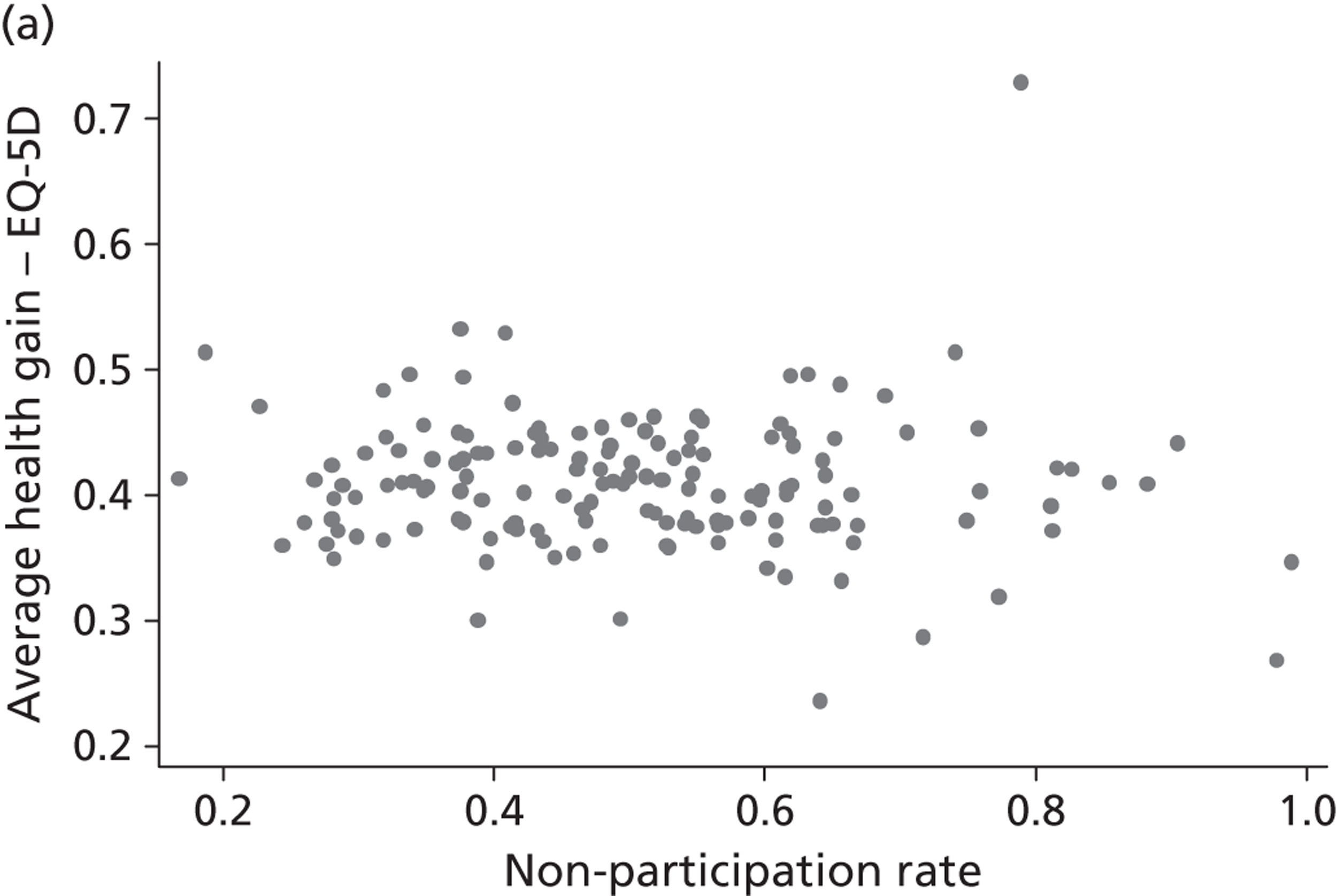
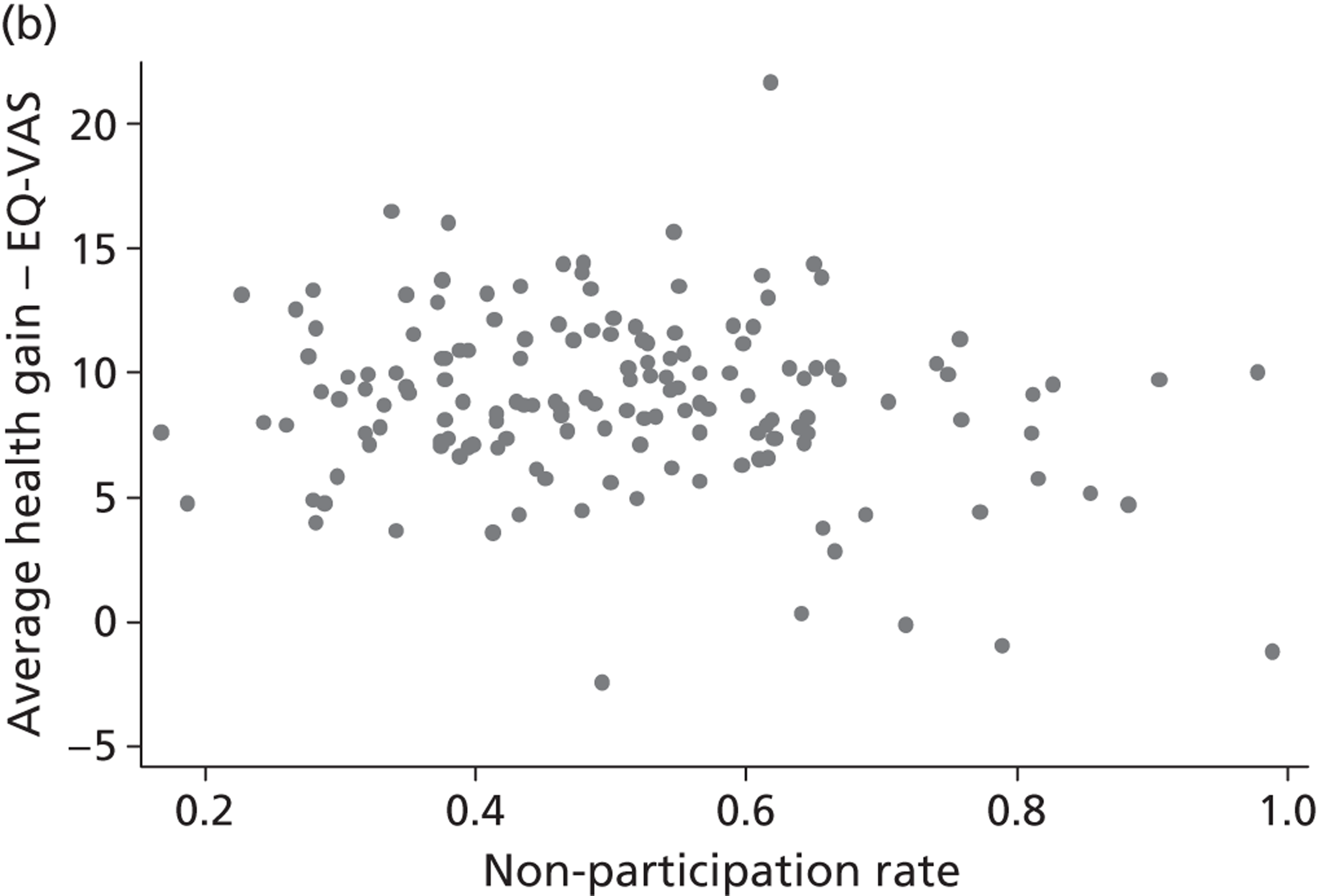
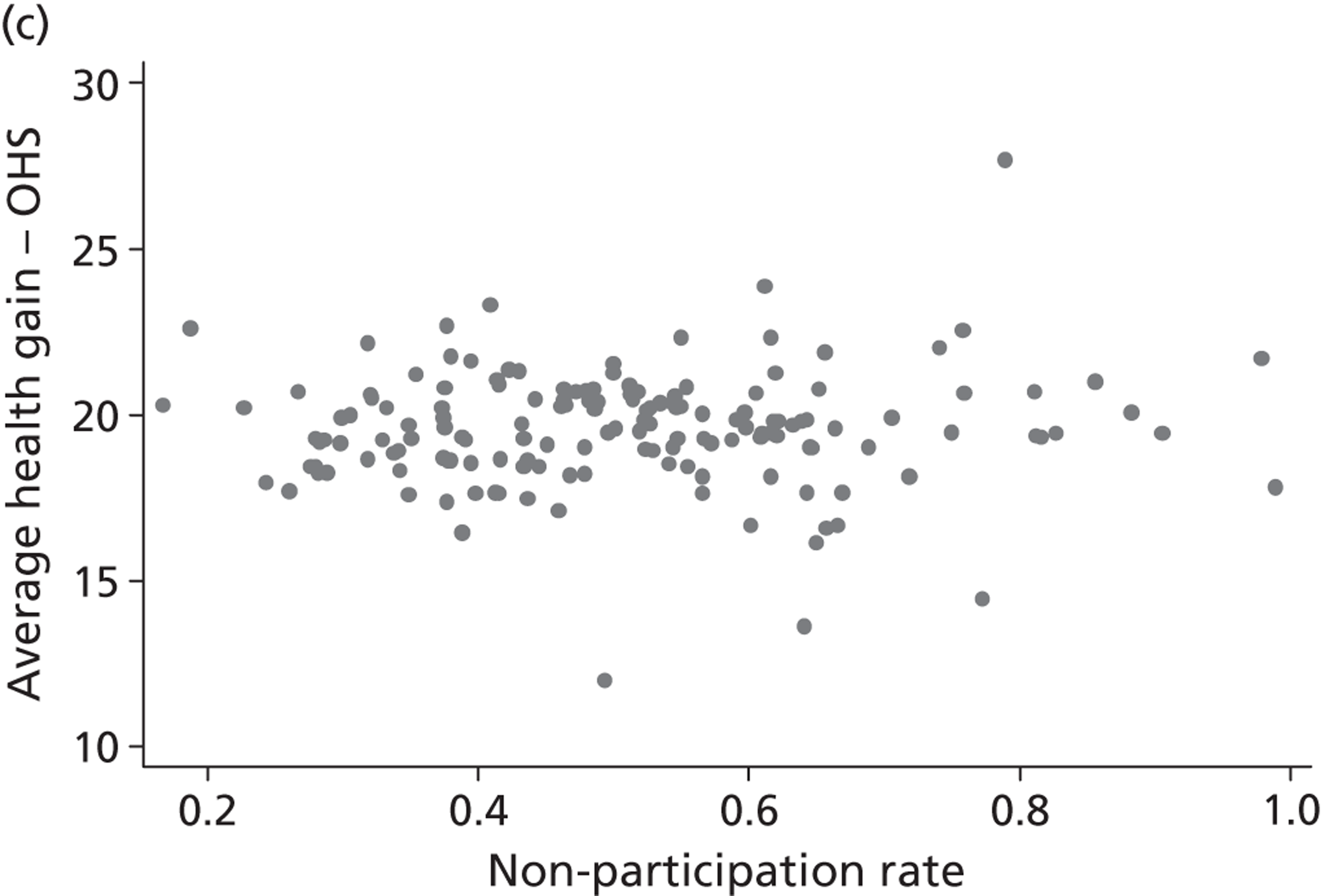
FIGURE 18.
Non-response rates and health outcome – knee replacement. (a) Non-response rate vs. EQ-5D health gain; (b) non-response rate vs. EQ-VAS health gain; and (c) non-response rate vs. OKS health gain.
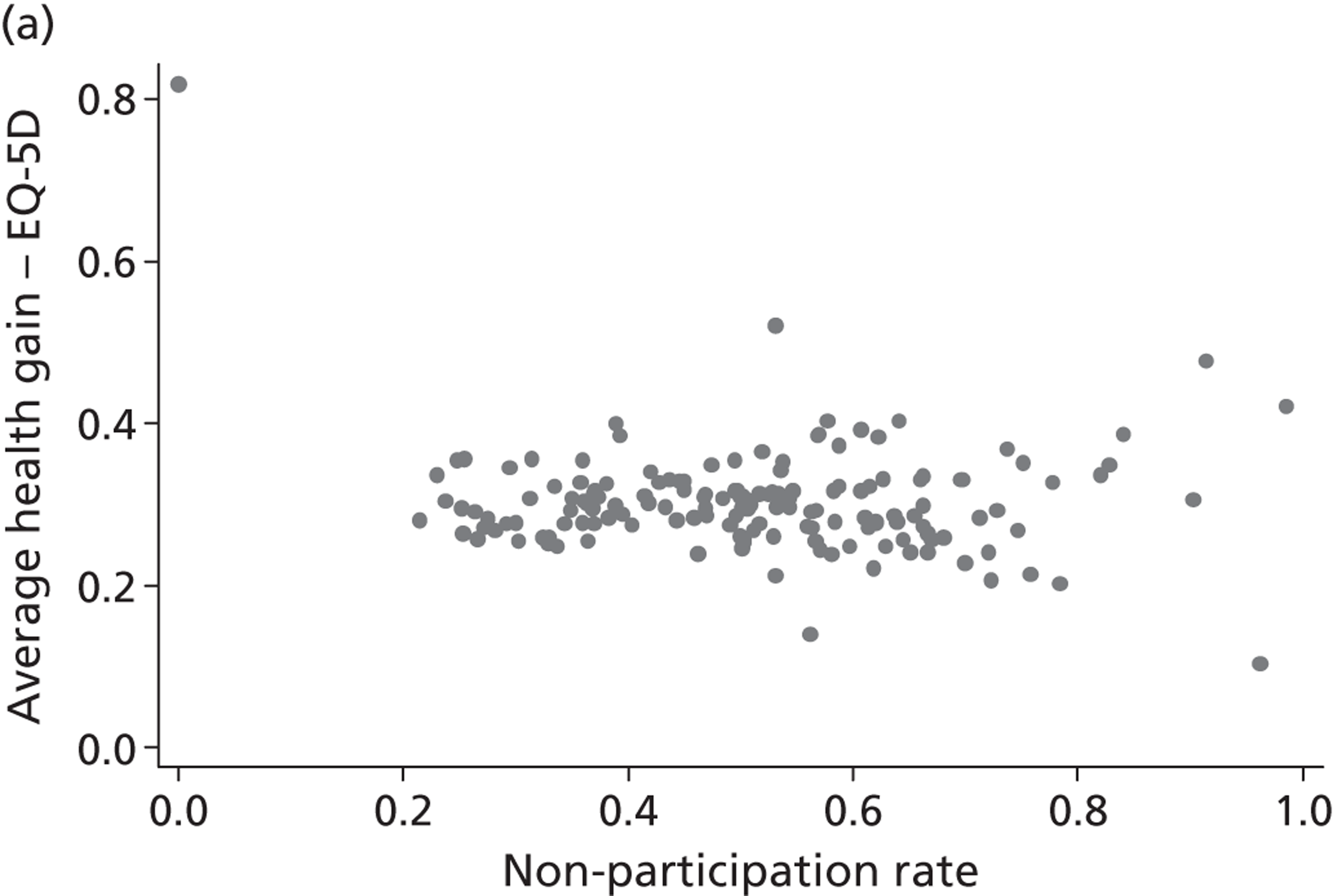
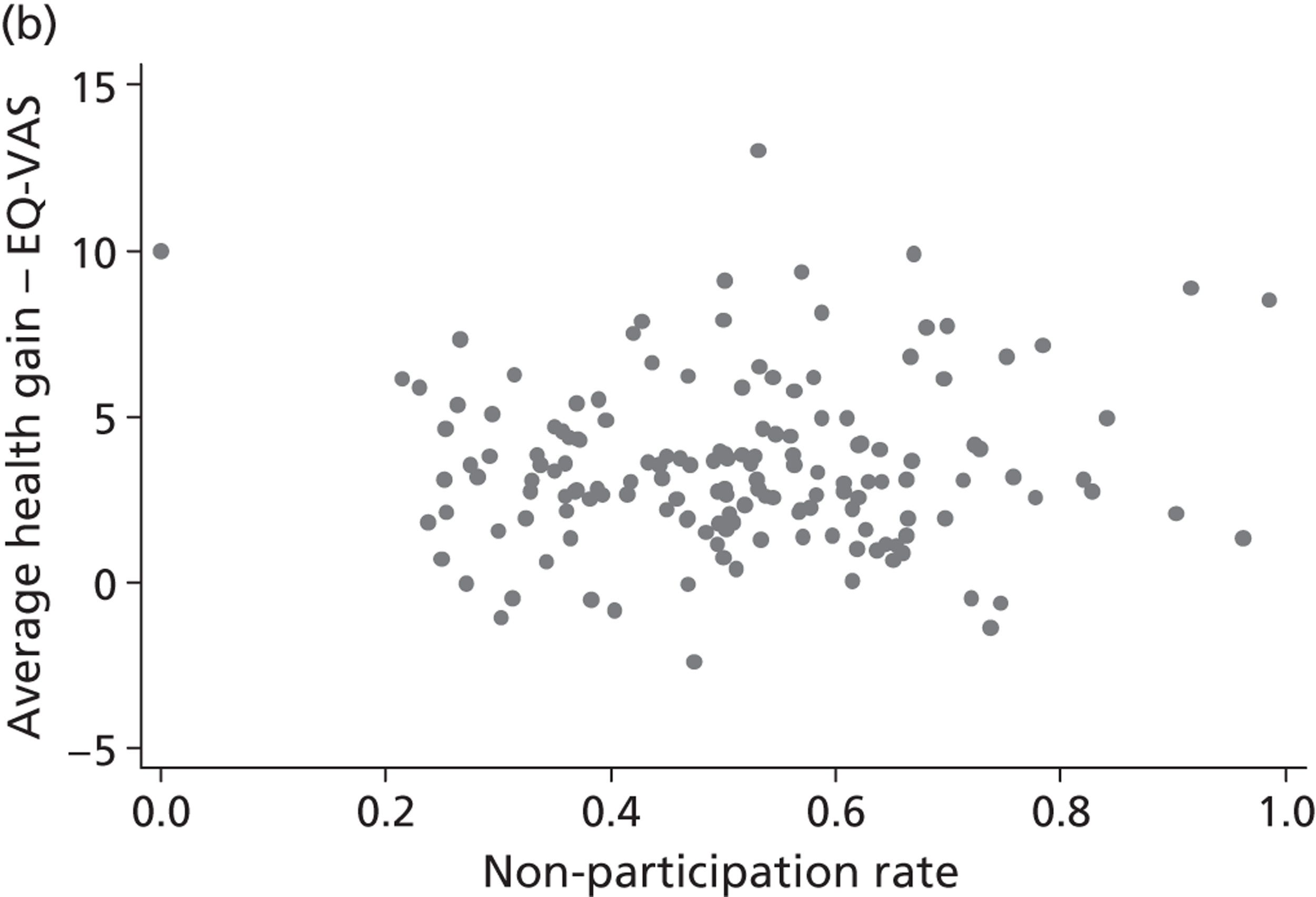
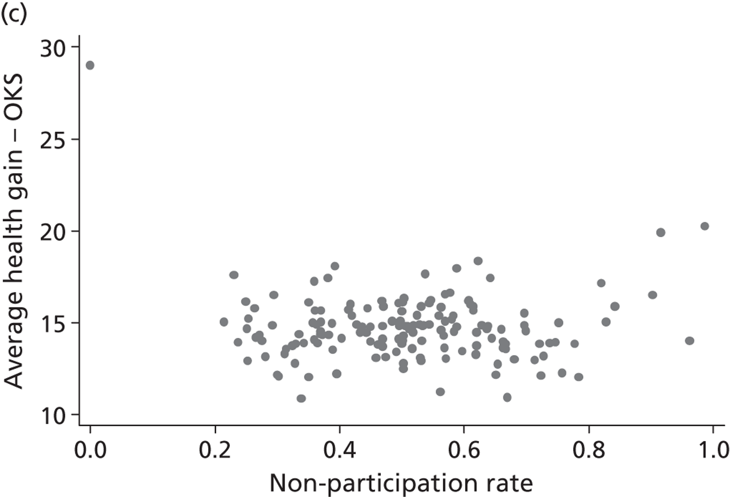
FIGURE 19.
Non-response rates and health outcome – groin hernia repair. (a) Non-response rate vs. EQ-5D health gain; and (b) non-response rate vs. EQ-VAS health gain.
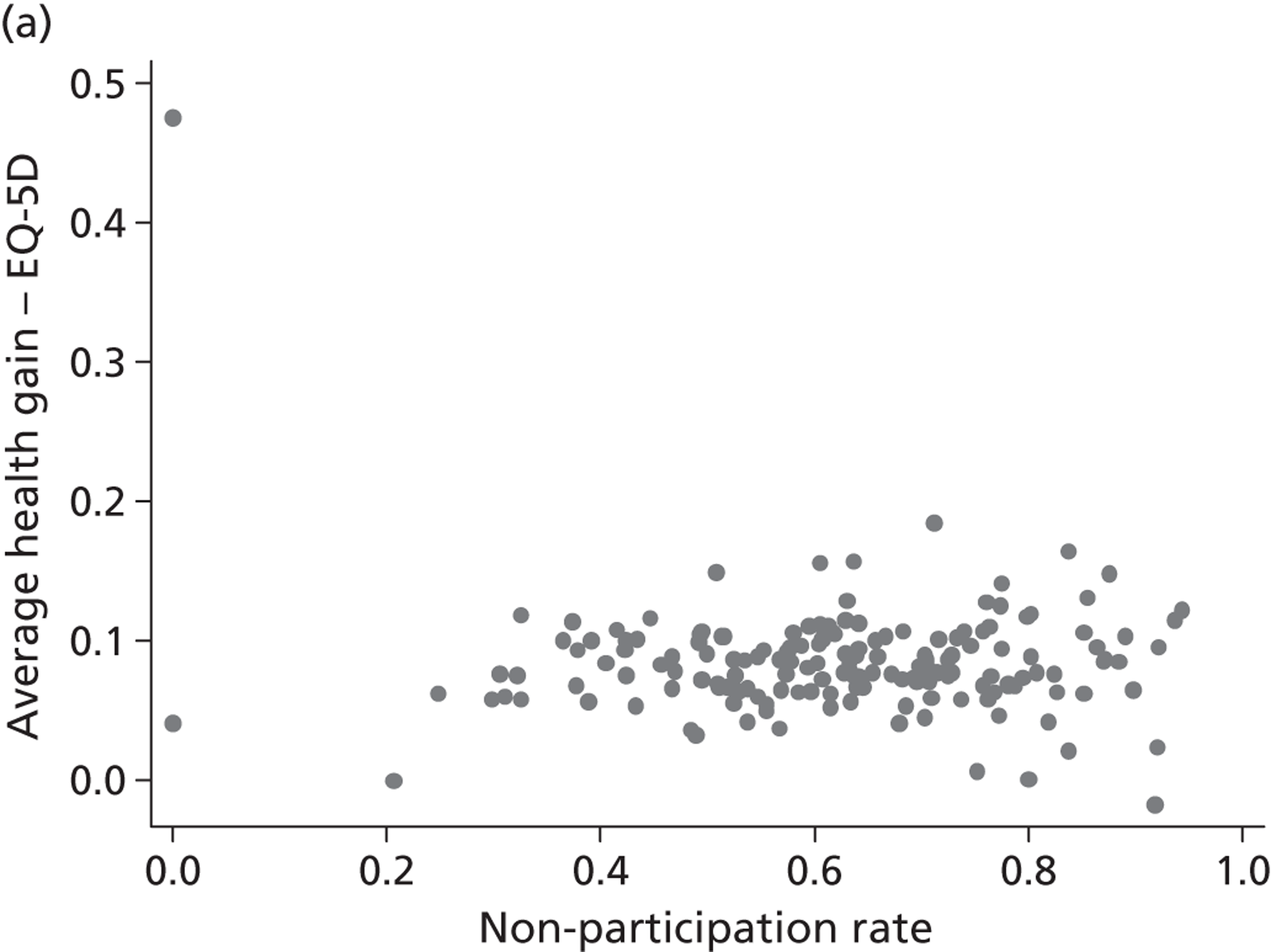
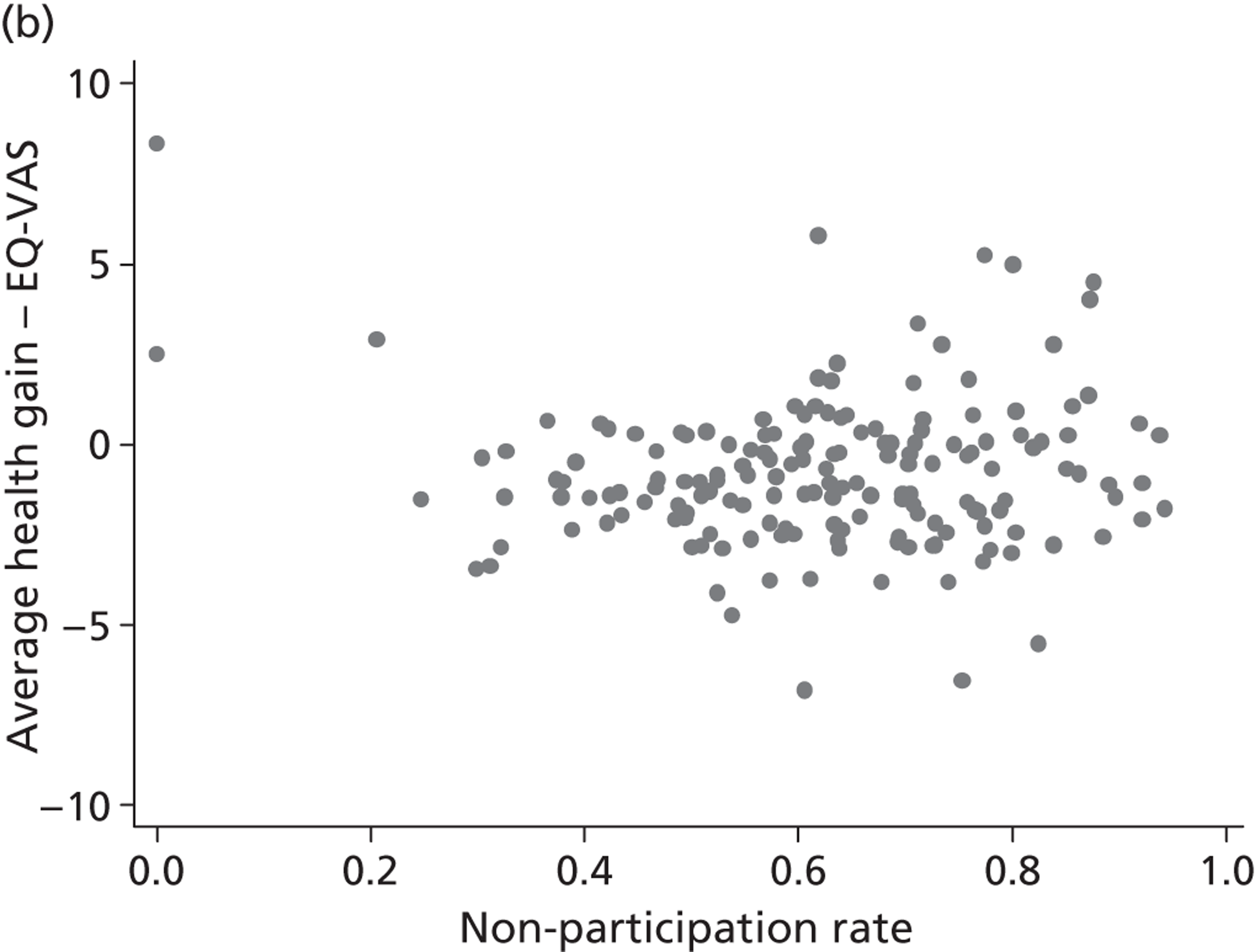
FIGURE 20.
Non-response rates and health outcome – varicose vein surgery. (a) Non-response rate vs. EQ-5D health gain; (b) non-response rate vs. EQ-VAS health gain; and (c) non-response rate vs. AVVQ health gain.
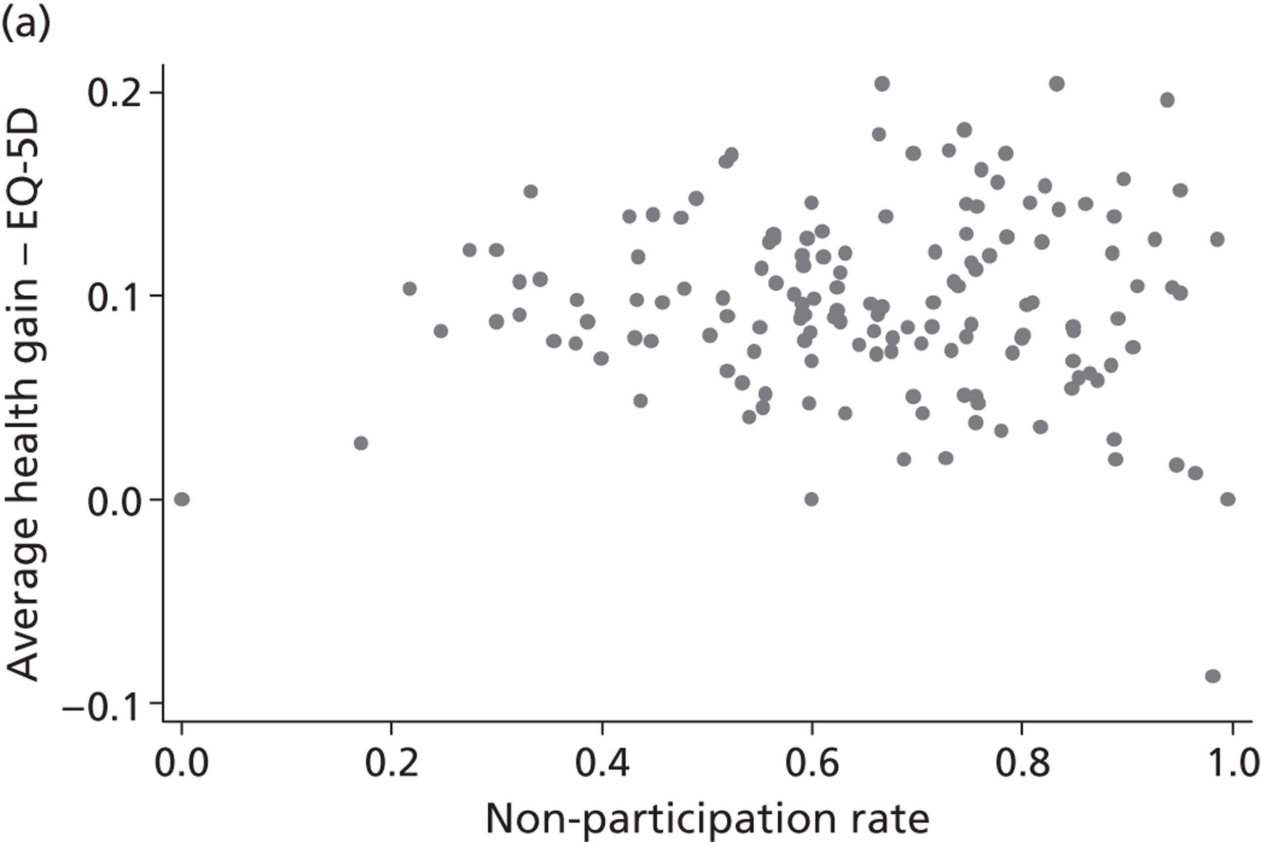
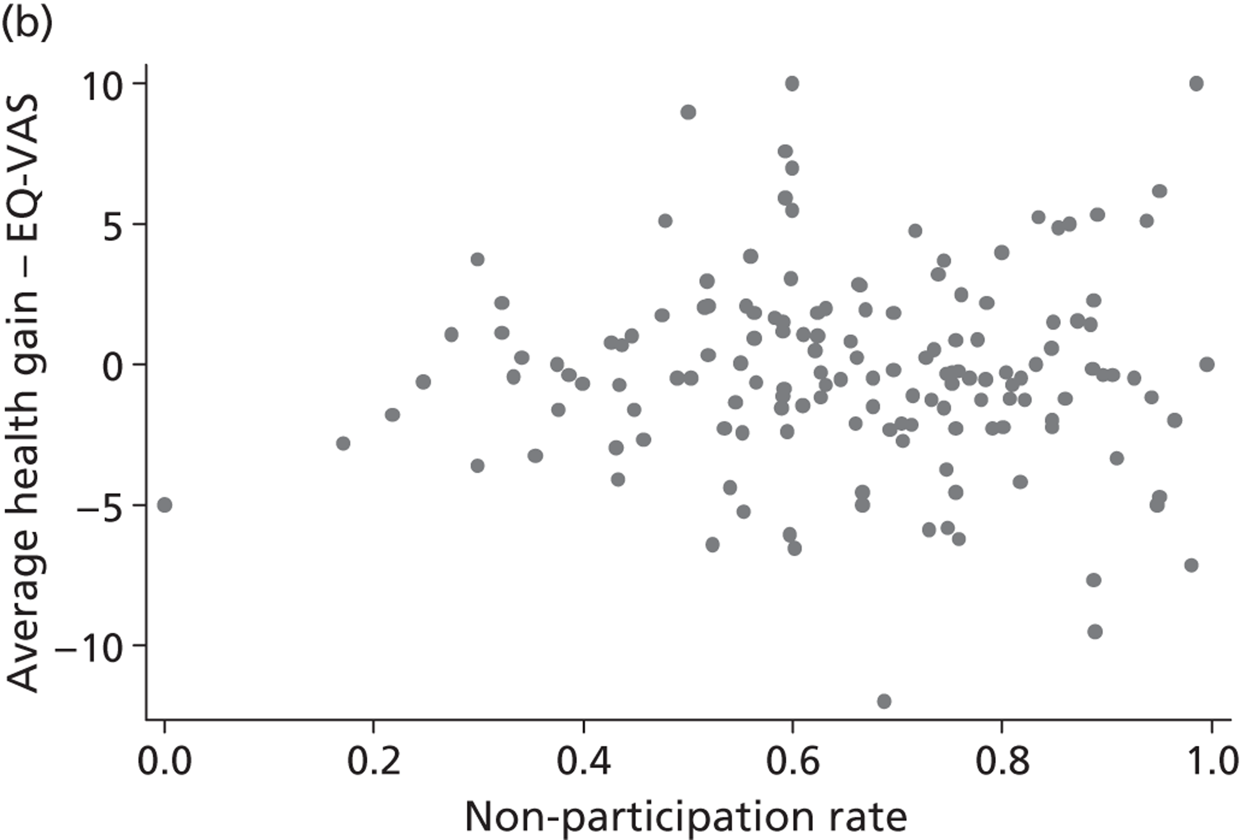
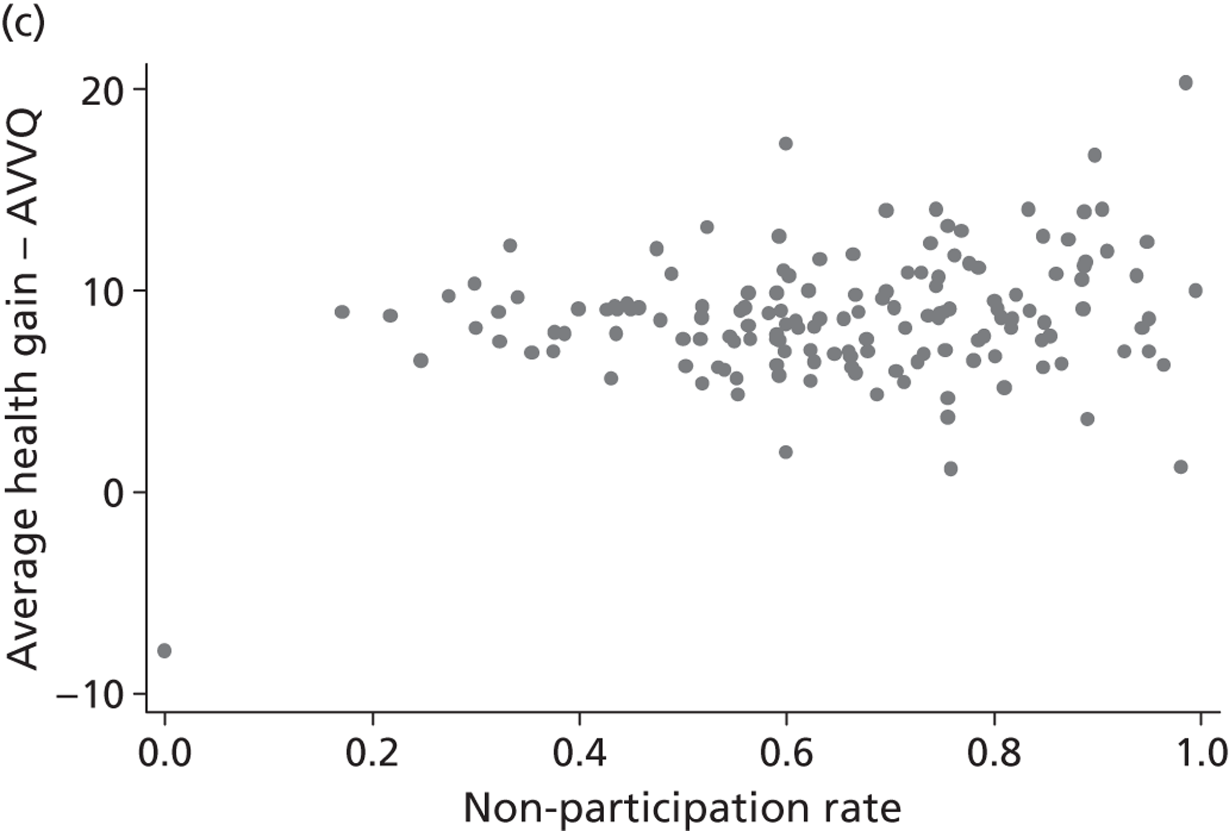
Estimation results
Unilateral hip replacement
Estimation results for those who had a hip replacement are presented in Table 12 . There are six sets of results, reflecting the different combinations of PRO instrument and resource use measure in the SUR model. The estimated effects of the explanatory variables on postoperative health status are not sensitive to the choice of resource use measure (cost of treatment or LoS). In contrast, the estimated impact on cost of treatment or LoS does appear slightly sensitive to the choice of PROM, this being because of how pretreatment health status is measured in these estimations.
| Measure of health | EQ-5D | EQ-5D | EQ-VAS | EQ-VAS | OHS | OHS | ||||||||||||
|---|---|---|---|---|---|---|---|---|---|---|---|---|---|---|---|---|---|---|
| Measure of resource use | LoS | Cost of treatment | LoS | Cost of treatment | LoS | Cost of treatment | ||||||||||||
| Health outcomesa | ||||||||||||||||||
| β | SE | β | SE | β | SE | β | SE | β | SE | β | SE | |||||||
| constant | 0.72 | 0.01 | *** | 0.72 | 0.01 | *** | 64.85 | 0.99 | *** | 64.85 | 0.99 | *** | 35.04 | 0.51 | *** | 35.05 | 0.51 | *** |
| age | 0.00 | 0.00 | 0.00 | 0.00 | – 0.06 | 0.01 | *** | – 0.06 | 0.01 | *** | – 0.01 | 0.01 | * | – 0.01 | 0.01 | * | ||
| male | 0.02 | 0.00 | *** | 0.02 | 0.00 | *** | 0.85 | 0.26 | ** | 0.85 | 0.26 | ** | 0.87 | 0.14 | *** | 0.87 | 0.14 | *** |
| wcharlson | – 0.03 | 0.00 | *** | – 0.03 | 0.00 | *** | – 2.64 | 0.21 | *** | – 2.64 | 0.21 | *** | – 0.68 | 0.11 | *** | – 0.68 | 0.11 | *** |
| add_diagnoses | – 0.01 | 0.00 | *** | – 0.01 | 0.00 | *** | – 1.26 | 0.08 | *** | – 1.25 | 0.08 | *** | – 0.55 | 0.04 | *** | – 0.54 | 0.04 | *** |
| revision | – 0.11 | 0.01 | *** | – 0.11 | 0.01 | *** | – 3.93 | 0.50 | *** | – 3.92 | 0.50 | *** | – 5.89 | 0.26 | *** | – 5.89 | 0.26 | *** |
| deprivation | – 0.21 | 0.02 | *** | – 0.21 | 0.02 | *** | – 12.74 | 1.41 | *** | – 12.66 | 1.41 | *** | – 9.81 | 0.74 | *** | – 9.77 | 0.74 | *** |
| multiepi | – 0.04 | 0.02 | ** | – 0.04 | 0.02 | ** | – 2.35 | 1.13 | * | – 2.40 | 1.13 | * | – 1.48 | 0.58 | * | – 1.50 | 0.58 | ** |
| initial health status | 0.22 | 0.01 | *** | 0.22 | 0.01 | *** | 0.28 | 0.01 | *** | 0.28 | 0.01 | *** | 0.34 | 0.01 | *** | 0.34 | 0.01 | *** |
| volume | 0.00 | 0.00 | * | 0.00 | 0.00 | * | 0.00 | 0.00 | 0.00 | 0.00 | * | 0.00 | 0.00 | 0.00 | 0.00 | |||
| teaching hospital | – 0.02 | 0.01 | * | – 0.02 | 0.01 | * | – 0.24 | 0.50 | – 0.27 | 0.51 | – 0.06 | 0.29 | – 0.05 | 0.30 | ||||
| Resource usea | ||||||||||||||||||
| constant | 0.77 | 0.23 | *** | 5.96 | 0.25 | *** | 1.21 | 0.24 | *** | 5.98 | 0.25 | *** | 1.21 | 0.23 | *** | 5.98 | 0.25 | *** |
| age | 0.07 | 0.00 | *** | 0.00 | 0.00 | 0.07 | 0.00 | *** | 0.00 | 0.00 | 0.07 | 0.00 | *** | 0.00 | 0.00 | |||
| male | – 0.40 | 0.05 | *** | 0.01 | 0.02 | – 0.41 | 0.05 | *** | 0.01 | 0.02 | – 0.36 | 0.05 | *** | 0.01 | 0.02 | |||
| wcharlson | 0.27 | 0.04 | *** | – 0.02 | 0.01 | 0.26 | 0.04 | *** | – 0.02 | 0.01 | 0.26 | 0.04 | *** | – 0.02 | 0.01 | |||
| add_diagnoses | 0.44 | 0.02 | *** | 0.06 | 0.01 | *** | 0.44 | 0.02 | *** | 0.06 | 0.01 | *** | 0.44 | 0.02 | *** | 0.06 | 0.01 | *** |
| revision | 4.91 | 0.25 | *** | 1.09 | 0.08 | *** | 4.91 | 0.25 | *** | 1.09 | 0.08 | *** | 4.93 | 0.25 | *** | 1.09 | 0.08 | *** |
| deprivation | 0.91 | 0.30 | ** | – 0.15 | 0.10 | 1.08 | 0.30 | *** | – 0.14 | 0.10 | 0.81 | 0.30 | ** | – 0.15 | 0.10 | |||
| multiepi | 5.55 | 0.23 | *** | 0.75 | 0.08 | *** | 5.51 | 0.23 | *** | 0.75 | 0.08 | *** | 5.55 | 0.23 | *** | 0.75 | 0.08 | *** |
| HRG2 | 0.35 | 0.14 | ** | 0.63 | 0.05 | *** | 0.34 | 0.14 | * | 0.63 | 0.05 | *** | 0.36 | 0.14 | ** | 0.63 | 0.05 | *** |
| HRG3 | – 2.45 | 0.28 | *** | 0.05 | 0.10 | – 2.46 | 0.28 | *** | 0.05 | 0.10 | – 2.42 | 0.28 | *** | 0.06 | 0.10 | |||
| HRG4 | 3.70 | 0.15 | *** | 2.22 | 0.05 | *** | 3.74 | 0.15 | *** | 2.22 | 0.05 | *** | 3.69 | 0.15 | *** | 2.22 | 0.05 | *** |
| HRG5 | – 3.22 | 0.30 | *** | – 0.44 | 0.10 | *** | – 3.26 | 0.30 | *** | – 0.45 | 0.10 | *** | – 3.18 | 0.30 | *** | – 0.44 | 0.10 | *** |
| HRG other | 1.50 | 0.16 | *** | 1.08 | 0.05 | *** | 1.52 | 0.16 | *** | 1.08 | 0.05 | *** | 1.51 | 0.16 | *** | 1.08 | 0.05 | *** |
| initial health status | – 0.96 | 0.09 | *** | – 0.06 | 0.03 | * | – 0.01 | 0.00 | *** | – 0.00 | 0.00 | – 0.04 | 0.00 | *** | – 0.00 | 0.00 | * | |
| volume | – 0.00 | 0.00 | ** | – 0.00 | 0.00 | – 0.00 | 0.00 | ** | – 0.00 | 0.00 | – 0.00 | 0.00 | ** | – 0.00 | 0.00 | |||
| teaching hospital | 0.49 | 0.22 | * | 0.50 | 0.38 | 0.46 | 0.21 | * | 0.50 | 0.38 | 0.50 | 0.21 | * | 0.50 | 0.38 | |||
| Variance components – hospital level | ||||||||||||||||||
| σ2 γ,h | 0.00 | 0.00 | *** | 0.00 | 0.00 | *** | 1.70 | 0.49 | *** | 1.80 | 0.51 | *** | 0.74 | 0.17 | *** | 0.78 | 0.18 | *** |
| cov(γ h , γ c ) = ρ 2 | – 0.00 | 0.00 | – 0.01 | 0.00 | – 0.17 | 0.16 | – 0.71 | 0.30 | * | – 0.16 | 0.09 | – 0.30 | 0.18 | |||||
| σ2 γ,c | 0.68 | 0.10 | *** | 2.70 | 0.32 | *** | 0.68 | 0.10 | *** | 2.70 | 0.32 | *** | 0.67 | 0.10 | *** | 2.70 | 0.32 | *** |
| Variance components – patient level | ||||||||||||||||||
| σ2 ε,h | 0.06 | 0.00 | *** | 0.06 | 0.00 | *** | 271.84 | 3.01 | *** | 271.80 | 3.01 | *** | 72.02 | 0.80 | *** | 72.01 | 0.80 | *** |
| cov(ε h , ε c ) = ρ 1 | – 0.07 | 0.01 | *** | – 0.00 | 0.00 | – 3.34 | 0.44 | *** | 0.07 | 0.15 | – 2.93 | 0.23 | *** | – 0.21 | 0.08 | ** | ||
| σ2 ε,c | 11.48 | 0.13 | *** | 1.29 | 0.010.00 | *** | 11.47 | 0.13 | *** | 1.29 | 0.01 | *** | 11.45 | 0.13 | *** | 1.29 | 0.01 | *** |
| n | 16,403 | 16,403 | 16,403 | 16,403 | 16,403 | 16,403 | ||||||||||||
In general, significant predictors of post-treatment health are not sensitive to the choice of PROM. As would be expected, post-treatment health status is negatively related to the weighted Charlson score, the number of diagnoses, revision surgery and higher neighbourhood deprivation; whereas, it is positively related to being of male gender and pretreatment health status. The impact of age on post-treatment health status is negative and significant when the EQ-VAS or OHS are considered, but insignificant when post-treatment health status is measured by the EQ-5D. The number of patients treated has a positive and significant association with post-treatment health in three of the six models.
With regard to resource use measures, older age, being of male gender, deprivation and higher weighted Charlson index are positive and statistically significant predictors of LoS but are unrelated to cost of treatment. Both LoS and cost of treatment are higher, and have a positive and significant relationship, for those who have a greater number of diagnoses and if a revision surgery is performed. As expected, there are also significant differences in resource use related to the HRG to which patients are allocated. The direction and size of these differences are consistent with the tariff payments for these HRGs (not presented in this report). Resource use is lower and, therefore, negatively related to patients presenting with a better state of pretreatment health. The number of patients treated has a negative and statistically significant relationship with LoS but not cost of treatment, whereas teaching activity of the hospital has a positive and statistically significant relationship with LoS but not cost of treatment.
After controlling for patient characteristics, there remains significant unexplained variation at patient level in terms of post-treatment health status and resource use, however these are measured. This is indicated by the significance (based on two-sided Wald tests) of σ ε , h 2 for outcomes, and σ ε , c 2 for resource use. The covariance between unobserved factors at patient level is negative, i.e. ρ 1 < 0, when LoS is considered (any PROM) or cost of treatment (only OHS). This suggests that common, unobserved patient characteristics exist that have a positive effect on post-treatment health status and that reduce the amount of resources used (and vice versa). However, this also suggests that there may be less variability in both generic PROMs and cost of treatment than in the condition-specific OHS and LoS.
At the hospital level, we find a similar pattern with both σ γ , h 2 and σ γ , c 2 being statistically significant. The estimated covariance between the hospital effects in each equation is always negative, independent of how resource use or PROs are measured. However, the covariance estimate is only statistically significant in the EQ-VAS/LoS model. Note that the size of the estimated variance components σ γ , h 2 differs across PROMs not least because of the scale of the instrument in question (e.g. the EQ-5D ranges from – 0.542 to 1 and the EQ-VAS ranges from 0 to 100).
Unilateral knee replacement
Table 13 presents the regression results for knee replacement surgery. The predictors of post-treatment health status for those having a knee replacement have the same sign (direction of influence) as the predictors of post-treatment health status following hip replacement surgery. Patients report lower post-treatment health status if they have a higher Charlson score, a greater number of diagnoses and live in more deprived areas, whereas men and those with higher pretreatment health status report better post-treatment health status. In contrast to the hip replacement results, age has a positive and statistically significant association with better post-treatment health status following knee replacement. No effects are identified regarding number of patients treated or teaching activity of the hospital. The direction and significance of the variables predicting LoS and cost of treatment for patients undergoing knee replacement are broadly consistent with those for patients having hip replacement.
In general, the variance and covariance parameters at patient level tell a similar story to those for the hip replacement sample. The variance terms at hospital level are statically significant, indicating systematic variation in both health outcomes and resource use across hospitals. However, the covariance terms are statistically insignificant other than for the EQ-VAS and LoS, providing little evidence for a systematic association between hospital performance in terms of resource use and quality of care.
| Measure of health | EQ-5D | EQ-5D | EQ-VAS | EQ-VAS | OKS | OKS | ||||||||||||
|---|---|---|---|---|---|---|---|---|---|---|---|---|---|---|---|---|---|---|
| Measure of resource use | LoS | Cost of treatment | LoS | Cost of treatment | LoS | Cost of treatment | ||||||||||||
| Health outcomesa | ||||||||||||||||||
| β | SE | β | SE | β | SE | β | SE | β | SE | β | SE | |||||||
| constant | 0.45 | 0.02 | *** | 0.45 | 0.02 | *** | 43.34 | 1.11 | *** | 43.33 | 1.11 | *** | 21.49 | 0.59 | *** | 21.48 | 0.59 | *** |
| age | 0.00 | 0.00 | *** | 0.00 | 0.00 | *** | 0.09 | 0.01 | *** | 0.09 | 0.01 | *** | 0.08 | 0.01 | *** | 0.08 | 0.01 | *** |
| male | 0.01 | 0.00 | ** | 0.01 | 0.00 | ** | 1.46 | 0.25 | *** | 1.46 | 0.25 | *** | 0.31 | 0.14 | * | 0.31 | 0.14 | * |
| wcharlson | – 0.02 | 0.00 | *** | – 0.02 | 0.00 | *** | – 2.19 | 0.19 | *** | – 2.18 | 0.19 | *** | – 0.60 | 0.10 | *** | – 0.60 | 0.10 | *** |
| add_diagnoses | – 0.01 | 0.00 | *** | – 0.01 | 0.00 | *** | – 0.95 | 0.07 | *** | – 0.94 | 0.07 | *** | – 0.41 | 0.04 | *** | – 0.40 | 0.04 | *** |
| revision | – 0.12 | 0.01 | *** | – 0.12 | 0.01 | *** | – 5.41 | 0.60 | *** | – 5.43 | 0.60 | *** | – 5.84 | 0.33 | *** | – 5.84 | 0.33 | *** |
| deprivation | – 0.20 | 0.02 | *** | – 0.20 | 0.02 | *** | – 12.63 | 1.28 | *** | – 12.55 | 1.28 | *** | – 8.92 | 0.71 | *** | – 8.87 | 0.71 | *** |
| multiepi | – 0.03 | 0.02 | – 0.03 | 0.02 | – 1.82 | 1.20 | – 1.84 | 1.20 | – 0.29 | 0.66 | – 0.30 | 0.66 | ||||||
| initial health status | 0.26 | 0.01 | *** | 0.26 | 0.01 | *** | 0.39 | 0.01 | *** | 0.39 | 0.01 | *** | 0.48 | 0.01 | *** | 0.48 | 0.01 | *** |
| volume | 0.00 | 0.00 | 0.00 | 0.00 | – 0.00 | 0.00 | – 0.00 | 0.00 | 0.00 | 0.00 | 0.00 | 0.00 | ||||||
| teaching hospital | 0.00 | 0.01 | 0.00 | 0.01 | 0.01 | 0.49 | 0.06 | 0.50 | – 0.04 | 0.31 | – 0.05 | 0.31 | ||||||
| Resource usea | ||||||||||||||||||
| constant | 0.71 | 0.23 | ** | 6.26 | 0.27 | *** | 1.29 | 0.24 | *** | 6.29 | 0.28 | *** | 1.17 | 0.23 | *** | 6.29 | 0.27 | *** |
| age | 0.07 | 0.00 | *** | 0.00 | 0.00 | ** | 0.07 | 0.00 | *** | 0.00 | 0.00 | ** | 0.07 | 0.00 | *** | 0.00 | 0.00 | ** |
| male | – 0.28 | 0.05 | *** | 0.01 | 0.02 | – 0.28 | 0.05 | *** | 0.01 | 0.02 | – 0.20 | 0.05 | *** | 0.02 | 0.02 | |||
| wcharlson | 0.25 | 0.04 | *** | – 0.02 | 0.01 | 0.23 | 0.04 | *** | – 0.02 | 0.01 | 0.24 | 0.04 | *** | – 0.02 | 0.01 | |||
| add_diagnoses | 0.34 | 0.01 | *** | 0.03 | 0.01 | *** | 0.34 | 0.01 | *** | 0.03 | 0.01 | *** | 0.34 | 0.01 | *** | 0.03 | 0.01 | *** |
| revision | 1.21 | 0.12 | *** | 0.12 | 0.04 | ** | 1.25 | 0.12 | *** | 0.12 | 0.04 | ** | 1.17 | 0.12 | *** | 0.12 | 0.04 | ** |
| deprivation | 0.84 | 0.25 | *** | 0.00 | 0.09 | 0.92 | 0.25 | *** | 0.01 | 0.09 | 0.70 | 0.25 | ** | – 0.01 | 0.09 | |||
| multiepi | 3.79 | 0.22 | *** | 0.14 | 0.08 | 3.82 | 0.22 | *** | 0.14 | 0.08 | 3.78 | 0.22 | *** | 0.14 | 0.08 | |||
| HRG2 | 0.76 | 0.11 | *** | 0.49 | 0.04 | *** | 0.73 | 0.11 | *** | 0.49 | 0.04 | *** | 0.75 | 0.11 | *** | 0.49 | 0.04 | *** |
| HRG3 | 3.89 | 0.12 | *** | 2.66 | 0.04 | *** | 3.92 | 0.12 | *** | 2.66 | 0.04 | *** | 3.89 | 0.11 | *** | 2.66 | 0.04 | *** |
| HRG4 | – 0.46 | 0.14 | ** | – 2.53 | 0.05 | *** | – 0.48 | 0.14 | *** | – 2.53 | 0.05 | *** | – 0.44 | 0.14 | ** | – 2.52 | 0.05 | *** |
| HRG5 | – 0.43 | 0.41 | 0.28 | 0.15 | – 0.29 | 0.41 | 0.29 | 0.15 | * | – 0.39 | 0.41 | 0.29 | 0.15 | * | ||||
| HRG other | 2.32 | 0.23 | *** | – 0.44 | 0.08 | *** | 2.36 | 0.23 | *** | – 0.44 | 0.08 | *** | 2.34 | 0.23 | *** | – 0.44 | 0.08 | *** |
| initial health status | – 0.85 | 0.08 | *** | – 0.05 | 0.03 | – 0.01 | 0.00 | *** | – 0.00 | 0.00 | – 0.04 | 0.00 | *** | – 0.00 | 0.00 | * | ||
| volume | – 0.00 | 0.00 | * | – 0.00 | 0.00 | – 0.00 | 0.00 | – 0.00 | 0.00 | – 0.00 | 0.00 | * | – 0.00 | 0.00 | ||||
| teaching hospital | 0.27 | 0.21 | – 0.09 | 0.41 | 0.25 | 0.20 | – 0.09 | 0.41 | 0.27 | 0.20 | – 0.09 | 0.41 | ||||||
| Variance components – hospital levela | ||||||||||||||||||
| σ2 γ,h | 0.00 | 0.00 | *** | 0.00 | 0.00 | *** | 1.66 | 0.47 | *** | 1.71 | 0.48 | *** | 0.84 | 0.19 | *** | 0.85 | 0.19 | *** |
| cov(γ h , γ c ) = ρ 2 | – 0.00 | 0.00 | – 0.00 | 0.00 | – 0.35 | 0.15 | * | – 0.18 | 0.31 | – 0.10 | 0.09 | – 0.27 | 0.19 | |||||
| σ2 γ,c | 0.64 | 0.09 | *** | 3.15 | 0.37 | *** | 0.63 | 0.09 | *** | 3.15 | 0.37 | *** | 0.63 | 0.09 | *** | 3.15 | 0.37 | *** |
| Variance components – patient levela | ||||||||||||||||||
| σ2 ε,h | 0.06 | 0.00 | *** | 0.06 | 0.00 | *** | 271.16 | 2.91 | *** | 271.12 | 2.91 | *** | 80.28 | 0.86 | *** | 80.28 | 0.86 | *** |
| cov(ε h , ε c ) = ρ 1 | – 0.08 | 0.01 | *** | – 0.00 | 0.00 | * | – 4.41 | 0.38 | *** | – 0.18 | 0.14 | – 3.15 | 0.21 | *** | – 0.08 | 0.07 | ||
| σ2 ε,c | 9.27 | 0.10 | *** | 1.18 | 0.01 | *** | 9.27 | 0.10 | *** | 1.18 | 0.01 | *** | 9.24 | 0.10 | *** | 1.17 | 0.01 | *** |
| n | 17,444 | 17,444 | 17,444 | 17,444 | 17,444 | 17,444 | ||||||||||||
Varicose vein surgery
Table 14 presents the regression results for varicose vein surgery, for which the health outcome models are broadly in line with those found for hip replacement and knee replacement. Post-treatment health status is negatively associated with age, weighted Charlson index, number of additional diagnoses and area deprivation; however, it is positively associated with being of male gender and initial health status, although the statistical significance of these effects is somewhat sensitive to the choice of PROM. With respect to resource use, we find that only the HRG to which the patient is assigned and the number of additional diagnoses are positive and statistically significant predictors for both LoS and cost of treatment.
| Measure of health | EQ-5D | EQ-5D | EQ-VAS | EQ-VAS | AVVQ | AVVQ | ||||||||||||
|---|---|---|---|---|---|---|---|---|---|---|---|---|---|---|---|---|---|---|
| Measure of resource use | LoS | Cost of treatment | LoS | Cost of treatment | LoS | Cost of treatment | ||||||||||||
| Health outcomesa | ||||||||||||||||||
| β | SE | β | SE | β | SE | β | SE | β | SE | β | SE | |||||||
| constant | 0.61 | 0.02 | *** | 0.61 | 0.02 | *** | 49.45 | 1.60 | *** | 49.44 | 1.60 | *** | 47.47 | 1.26 | *** | 47.44 | 1.26 | *** |
| age | – 0.00 | 0.00 | *** | – 0.00 | 0.00 | *** | – 0.12 | 0.02 | *** | – 0.12 | 0.02 | *** | – 0.02 | 0.01 | * | – 0.02 | 0.01 | |
| male | 0.01 | 0.01 | 0.01 | 0.01 | 0.07 | 0.46 | 0.07 | 0.46 | 1.38 | 0.27 | *** | 1.38 | 0.27 | *** | ||||
| wcharlson | – 0.01 | 0.01 | – 0.01 | 0.01 | – 3.29 | 0.75 | *** | – 3.30 | 0.75 | *** | – 0.76 | 0.43 | – 0.76 | 0.43 | ||||
| add_diagnoses | – 0.02 | 0.00 | *** | – 0.02 | 0.00 | *** | – 1.19 | 0.26 | *** | – 1.19 | 0.26 | *** | – 0.22 | 0.15 | – 0.22 | 0.15 | ||
| deprivation | – 0.13 | 0.03 | *** | – 0.13 | 0.03 | *** | – 7.91 | 2.10 | *** | – 7.99 | 2.10 | *** | – 0.40 | 1.24 | – 0.51 | 1.23 | ||
| multiepi | 0.12 | 0.06 | * | 0.12 | 0.06 | * | 5.53 | 4.75 | 5.50 | 4.75 | 0.61 | 2.77 | 0.62 | 2.77 | ||||
| initial health status | 0.43 | 0.01 | *** | 0.43 | 0.01 | *** | 0.49 | 0.01 | *** | 0.49 | 0.01 | *** | 0.53 | 0.01 | *** | 0.53 | 0.01 | *** |
| volume | – 0.00 | 0.00 | – 0.00 | 0.00 | 0.00 | 0.01 | 0.00 | 0.01 | – 0.01 | 0.00 | – 0.01 | 0.00 | ||||||
| teaching hospital | – 0.00 | 0.01 | – 0.00 | 0.01 | – 1.08 | 0.60 | – 1.06 | 0.60 | – 0.26 | 0.43 | – 0.20 | 0.41 | ||||||
| Resource usea | ||||||||||||||||||
| constant | 0.01 | 0.05 | 1.19 | 0.07 | *** | 0.01 | 0.06 | 1.18 | 0.07 | *** | 0.15 | 0.07 | * | 1.22 | 0.08 | *** | ||
| age | 0.00 | 0.00 | *** | 0.00 | 0.00 | 0.00 | 0.00 | *** | 0.00 | 0.00 | 0.00 | 0.00 | *** | 0.00 | 0.00 | |||
| male | 0.00 | 0.02 | 0.03 | 0.01 | * | 0.00 | 0.02 | 0.03 | 0.01 | * | 0.01 | 0.02 | 0.03 | 0.01 | ** | |||
| wcharlson | 0.03 | 0.03 | 0.02 | 0.02 | 0.03 | 0.03 | 0.02 | 0.02 | 0.03 | 0.03 | 0.02 | 0.02 | ||||||
| add_diagnoses | 0.05 | 0.01 | *** | 0.02 | 0.01 | ** | 0.05 | 0.01 | *** | 0.02 | 0.01 | ** | 0.05 | 0.01 | *** | 0.02 | 0.01 | ** |
| deprivation | 0.08 | 0.07 | – 0.02 | 0.06 | 0.09 | 0.07 | – 0.02 | 0.06 | 0.08 | 0.07 | – 0.02 | 0.06 | ||||||
| multiepi | 0.51 | 0.16 | ** | – 0.14 | 0.13 | 0.51 | 0.16 | *** | – 0.13 | 0.13 | 0.50 | 0.16 | ** | – 0.13 | 0.13 | |||
| HRG2 | 0.22 | 0.02 | *** | 0.20 | 0.02 | *** | 0.23 | 0.02 | *** | 0.20 | 0.02 | *** | 0.22 | 0.02 | *** | 0.19 | 0.02 | *** |
| HRG3 | 0.05 | 0.03 | – 0.08 | 0.03 | * | 0.05 | 0.03 | – 0.08 | 0.03 | * | 0.05 | 0.03 | – 0.08 | 0.03 | ** | |||
| HRG4 | 0.07 | 0.03 | * | 0.12 | 0.03 | *** | 0.07 | 0.03 | * | 0.12 | 0.03 | *** | 0.07 | 0.03 | * | 0.12 | 0.03 | *** |
| HRG5 | 0.56 | 0.08 | *** | 0.35 | 0.07 | *** | 0.55 | 0.08 | *** | 0.35 | 0.07 | *** | 0.55 | 0.08 | *** | 0.35 | 0.07 | *** |
| HRG other | 0.41 | 0.06 | *** | 0.21 | 0.05 | *** | 0.42 | 0.06 | *** | 0.22 | 0.05 | *** | 0.40 | 0.06 | *** | 0.21 | 0.05 | *** |
| initial health status | – 0.02 | 0.04 | – 0.03 | 0.03 | – 0.00 | 0.00 | – 0.00 | 0.00 | – 0.00 | 0.00 | * | – 0.00 | 0.00 | |||||
| volume | – 0.00 | 0.00 | – 0.00 | 0.00 | – 0.00 | 0.00 | – 0.00 | 0.00 | – 0.00 | 0.00 | – 0.00 | 0.00 | ||||||
| teaching hospital | – 0.02 | 0.04 | 0.05 | 0.11 | – 0.02 | 0.04 | 0.05 | 0.11 | – 0.02 | 0.04 | 0.05 | 0.11 | ||||||
| Variance components – hospital levela | ||||||||||||||||||
| σ2 γ,h | 0.00 | 0.00 | 0.00 | 0.00 | 1.04 | 0.77 | 0.96 | 0.76 | 1.18 | 0.42 | ** | 1.06 | 0.39 | ** | ||||
| cov(γ h , γ c ) | – 0.00 | 0.00 | 0.00 | 0.00 | 0.07 | 0.04 | 0.15 | 0.11 | 0.05 | 0.03 | 0.22 | 0.08 | ** | |||||
| (0.00) | (0.00) | (0.04) | (0.11) | (0.03) | (0.08) | |||||||||||||
| σ2 γ,c | 0.02 | 0.00 | *** | 0.20 | 0.03 | *** | 0.02 | 0.00 | *** | 0.20 | 0.03 | *** | 0.02 | 0.00 | *** | 0.20 | 0.03 | *** |
| Variance components – patient levela | ||||||||||||||||||
| σ2 ε,h | 0.03 | 0.00 | *** | 0.03 | 0.00 | *** | 178.57 | 4.15 | *** | 178.59 | 4.15 | *** | 60.15 | 1.40 | *** | 60.21 | 1.40 | *** |
| cov(ε h , ε c ) | 0.00 | 0.00 | – 0.00 | 0.00 | 0.05 | 0.10 | 0.09 | 0.08 | – 0.05 | 0.06 | – 0.03 | 0.05 | ||||||
| σ2 ε,c | 0.19 | 0.00 | *** | 0.14 | 0.00 | *** | 0.19 | 0.00 | *** | 0.14 | 0.00 | *** | 0.19 | 0.00 | *** | 0.14 | 0.00 | *** |
| n | 3772 | 3772 | 3772 | 3772 | 3772 | 3772 | ||||||||||||
With respect to the variance and covariance components, we make three interesting observations. First, the covariance term at patient level is always insignificant. This suggests that health outcome and resource use do not depend on common unobserved factors at patient level. Second, the variance component for the hospital effect in the health outcome equation is insignificant for both generic PROMs. Hence, both instruments do not pick up any systematic variation in health outcome across hospitals. In contrast, the estimated variance σ γ , h 2 is significant when health status is assessed by the AVVQ. Finally, the covariance terms at hospital level are positive and significant for the model considering the AVVQ and cost of treatment. Hence, there may be unobserved factors that are associated with both systematic variation in health outcomes and cost of treatment, leading to a positive correlation between the two.
Groin hernia repair
Bivariate response models, as described in Methodology and statistical approach, failed to estimate for the groin hernia repair model. This is because, after allowing for risk adjustment, there appears to be no systematic hospital variation with respect to the EQ-5D utility scores or the EQ-VAS scores. To study the effect of case-mix variables and hospital characteristics on costs and outcomes of treatment, we estimate these equations in isolation, i.e. constrain any correlation between the two objectives to be zero. The results of these univariate estimations for groin hernia repair are reported in Table 15 .
| Variablea | Health outcome | Resource use | ||||||||||
|---|---|---|---|---|---|---|---|---|---|---|---|---|
| EQ-5D | EQ-VAS | LoS | Cost of treatment | |||||||||
| β | SE | β | SE | β | SE | β | SE | |||||
| constant | 0.60 | 0.01 | *** | 36.86 | 1.08 | *** | 0.04 | 0.07 | 1.48 | 0.08 | *** | |
| age | – 0.00 | 0.00 | – 0.06 | 0.01 | *** | 0.01 | 0.00 | *** | 0.00 | 0.00 | *** | |
| male | 0.03 | 0.01 | *** | 0.61 | 0.49 | – 0.01 | 0.03 | 0.02 | 0.02 | |||
| wcharlson | – 0.02 | 0.00 | *** | – 2.47 | 0.27 | *** | 0.03 | 0.02 | 0.03 | 0.01 | ** | |
| add_diagnoses | – 0.01 | 0.00 | *** | – 0.77 | 0.10 | *** | 0.11 | 0.01 | *** | 0.03 | 0.00 | *** |
| deprivation | – 0.14 | 0.02 | *** | – 9.88 | 1.25 | *** | 0.07 | 0.09 | 0.07 | 0.05 | ||
| multiepi | – 0.00 | 0.02 | 0.32 | 1.82 | 1.65 | 0.12 | *** | 0.44 | 0.06 | *** | ||
| pre-treatment health status | 0.37 | 0.01 | *** | 0.60 | 0.01 | *** | – 0.24 | 0.04 | *** | – 0.10 | 0.02 | *** |
| HRG2 | – | – | – | – | 0.25 | 0.03 | *** | 0.09 | 0.01 | *** | ||
| HRG3 | – | – | – | – | 0.41 | 0.06 | *** | 0.28 | 0.03 | *** | ||
| HRG4 | – | – | – | – | 0.57 | 0.14 | *** | 0.43 | 0.07 | *** | ||
| HRG5 | – | – | – | – | 0.22 | 0.14 | – 0.03 | 0.07 | ||||
| HRG other | – | – | – | – | 0.99 | 0.07 | *** | 0.62 | 0.04 | *** | ||
| volume | – 0.00 | 0.00 | 0.00 | 0.00 | – 0.00 | 0.00 | – 0.00 | 0.00 | * | |||
| teaching hospital | 0.01 | 0.00 | 0.37 | 0.34 | 0.14 | 0.05 | *** | 0.13 | 0.12 | |||
| Variance components | ||||||||||||
| σ2 γ | 0.00 | – | 0.00 | – | 0.03 | 0.00 | *** | 0.28 | 0.03 | *** | ||
| σ2 ε | 0.03 | 0.00 | *** | 157.24 | 2.18 | *** | 0.66 | 0.01 | *** | 0.17 | 0.00 | *** |
| n | 10,389 | 10,389 | 10,389 | 10,389 | ||||||||
We find that patients reporting better pretreatment health also report higher post-treatment health, independent of whether this is measured by the EQ-5D or EQ-VAS. Post-treatment health status is negatively associated with the Charlson scores, the number of diagnoses and the area deprivation of the patient’s residence.
Cost of treatment and LoS are positively associated with age, the number of diagnoses and when more than one consultant provided care; however, they are negatively associated with the number of patients treated at the hospital. Patients who report better pretreatment health generate lower costs and have shorter stays in hospital.
The lack of systematic variation in health outcomes precludes benchmarking of relative hospital quality performance for groin hernia patients. However, there does appear to be scope for improved control of resource use as indicated by the positive values for σ γ , c 2 in both the cost of treatment and LoS equations.
Performance assessment
Identifying better/worse than expected performers
Table 16 presents the number of hospitals that are identified as being statistically significantly different from what would be expected given the characteristics of the hospital and its patients. The columns ‘Health outcome’ and ‘Resource use’ under the heading ‘Assessment by objective’ present the number of hospitals performing statistically significantly differently from the risk-adjusted average on each of these objectives when analysed in isolation. Results reported under the heading ‘Joint assessment of objectives’ reflect the joint performance of hospitals on both objectives. Accordingly, if a specific hospital performs better than expected in terms of health outcome but not in terms of resource use, it will not be considered a better than expected performer in terms of joint performance.
| Assessment by objective | |||||||||
|---|---|---|---|---|---|---|---|---|---|
| Health outcome | Resource usea | Joint assessment of objectives | |||||||
| Better than expected | Worse than expected | Total | Better than expected | Worse than expected | Total | Better than expected | Worse than expected | Total | |
| Hip replacement (142 hospitals) | |||||||||
| Cost of treatment | |||||||||
| EQ-5D utility score | 2 | 5 | 7 | 56 | 44 | 100 | 1 | 2 | 3 |
| EQ-VAS score | 1 | 3 | 4 | 56 | 44 | 100 | 1 | 2 | 3 |
| OHS | 3 | 6 | 9 | 56 | 44 | 100 | 2 | 3 | 5 |
| LoS | |||||||||
| EQ-5D utility score | 2 | 5 | 7 | 29 | 24 | 53 | 1 | 3 | 4 |
| EQ-VAS score | 0 | 3 | 3 | 29 | 23 | 52 | 0 | 2 | 2 |
| OHS | 4 | 6 | 10 | 29 | 24 | 53 | 1 | 4 | 5 |
| Knee replacement (143 hospitals) | |||||||||
| Cost of treatment | |||||||||
| EQ-5D utility score | 1 | 6 | 7 | 66 | 36 | 102 | 1 | 3 | 4 |
| EQ-VAS score | 2 | 4 | 6 | 66 | 36 | 102 | 1 | 2 | 3 |
| OKS | 6 | 5 | 11 | 67 | 36 | 103 | 4 | 2 | 6 |
| LoS | |||||||||
| EQ-5D utility score | 1 | 6 | 7 | 30 | 28 | 58 | 0 | 2 | 2 |
| EQ-VAS score | 2 | 3 | 5 | 29 | 27 | 56 | 2 | 1 | 3 |
| OKS | 6 | 5 | 11 | 30 | 28 | 58 | 2 | 1 | 3 |
| Groin hernia repair (146 hospitals) | |||||||||
| Cost of treatment | – | – | – | 10 | 17 | 27 | – | – | – |
| LoS | – | – | – | 10 | 17 | 27 | – | – | – |
| Varicose vein surgery (130 hospitals) | |||||||||
| Cost of treatment | |||||||||
| EQ-5D utility score | 0 | 0 | 0 | 47 | 35 | 82 | 0 | 0 | 0 |
| EQ-VAS score | 0 | 0 | 0 | 47 | 35 | 82 | 0 | 0 | 0 |
| AVVQ score | 1 | 3 | 4 | 48 | 35 | 83 | 0 | 0 | 0 |
| LoS | |||||||||
| EQ-5D utility score | 0 | 0 | 0 | 2 | 10 | 12 | 0 | 0 | 0 |
| EQ-VAS score | 1 | 0 | 1 | 1 | 10 | 11 | 0 | 0 | 0 |
| AVVQ score | 2 | 3 | 5 | 2 | 12 | 14 | 0 | 0 | 0 |
Three important results can be derived from Table 16 . First, a greater number of better/worse than expected hospitals, with respect to cost performance, are identified when resources are measured in terms of cost of treatment rather than LoS. Similarly, more hospitals are classified as performing significantly differently from the average when using condition-specific measures of health outcome instead of the generic EQ-5D or EQ-VAS. In both cases, this reflects the higher variability in unadjusted scores that carries through to the risk-adjusted performance estimates. Second, while many hospitals achieve better/worse results than expected on one of the two objectives, very few can be identified as performing well or badly on both objectives simultaneously. Third, no hospitals are identified as either better or worse than expected in terms of their performance when resource use and health outcomes are jointly assessed for varicose vein surgery. Because of this (and the earlier finding of a lack of systematic variation in health outcomes across hospitals for groin hernia patients), we focus on hip replacement and knee replacement in illustrating joint performance and in the remaining discussion.
Figures 21 and 22 present scatterplots of the performance estimates in the two-dimensional performance space for all six resource use and outcome measure combinations for hip replacement and knee replacement. Each point represents a hospital and we present CrIs for only those hospitals that are identified as better/worse than expected performers on both objectives simultaneously.
FIGURE 21.
Joint cost and quality performance estimates – hip replacement. (a) LoS/EQ-5D index; (b) LoS/EQ-VAS; (c) LoS/OHS; (d) cost of treatment/EQ-5D index; (e) cost of treatment/EQ-VAS; and (f) cost of treatment/OHS.
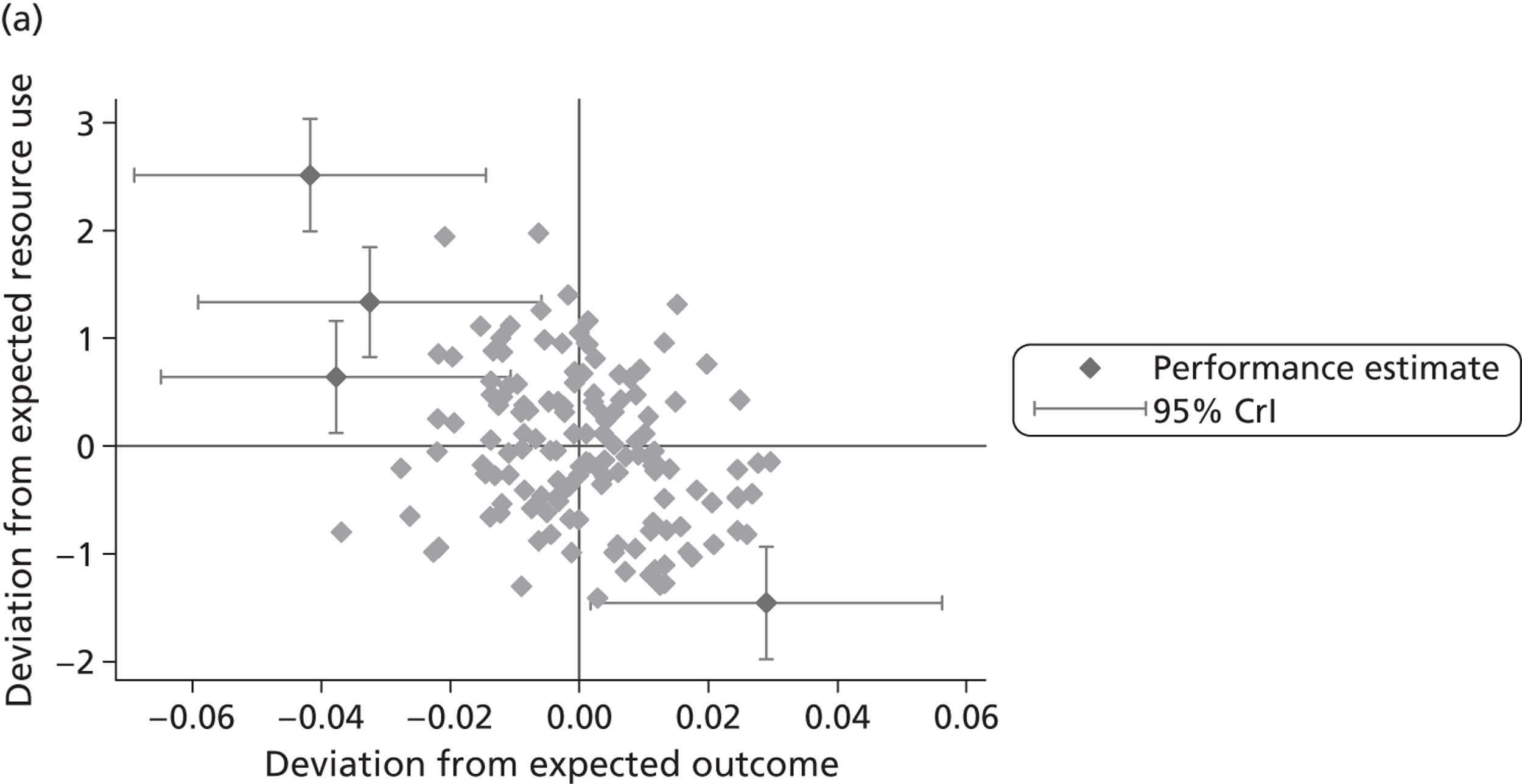
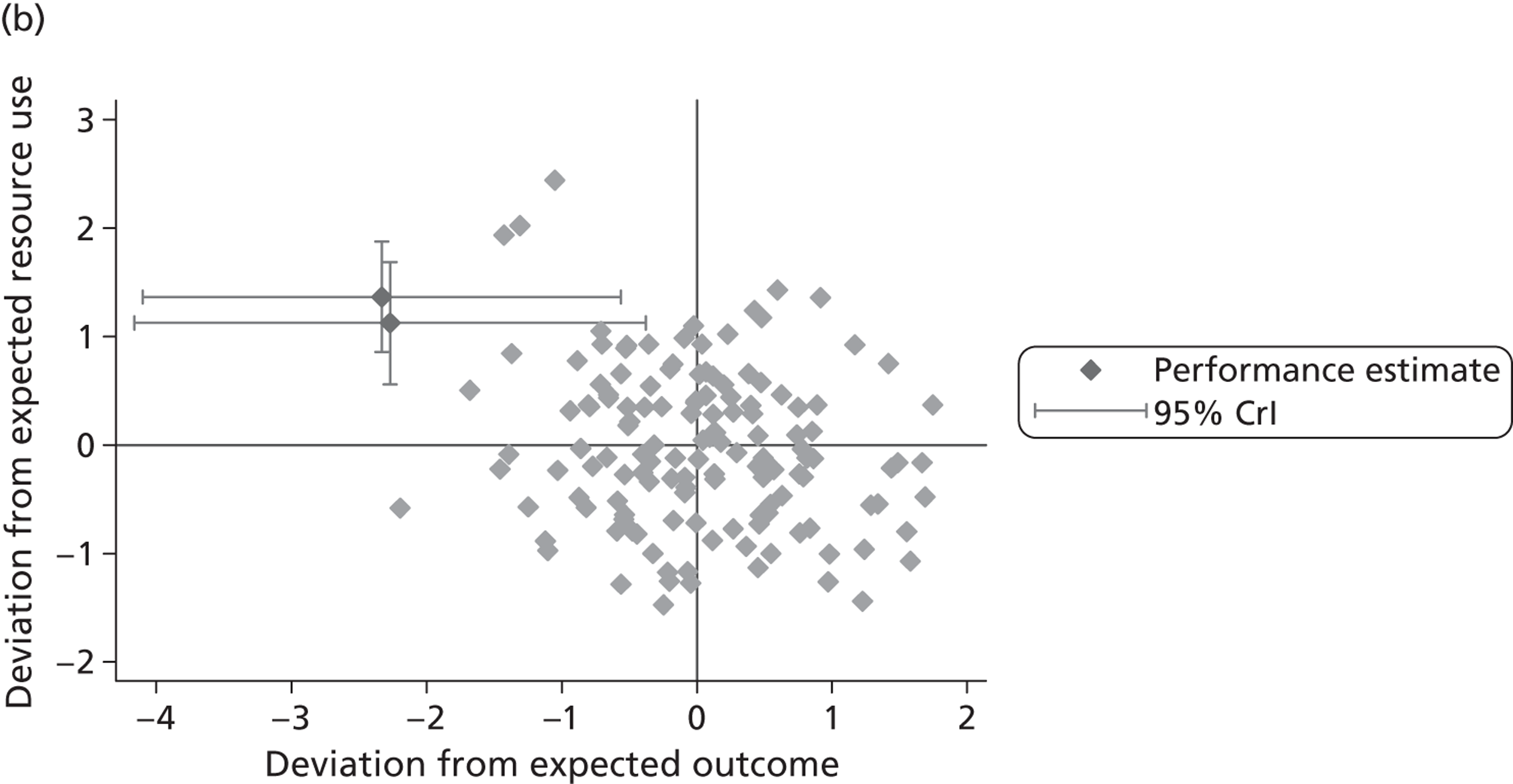
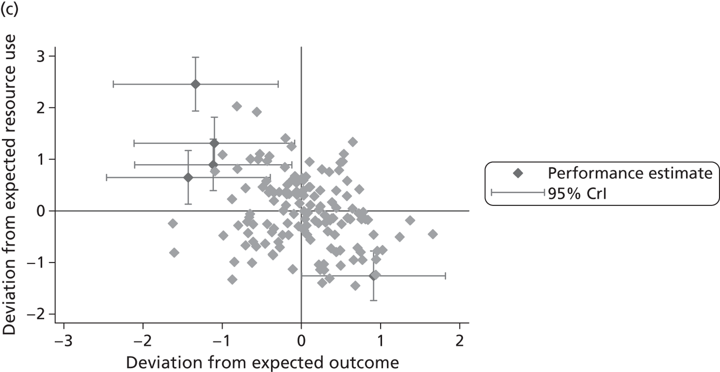
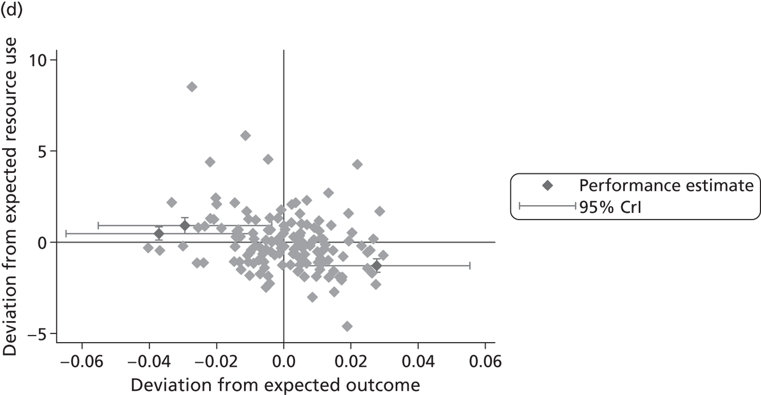
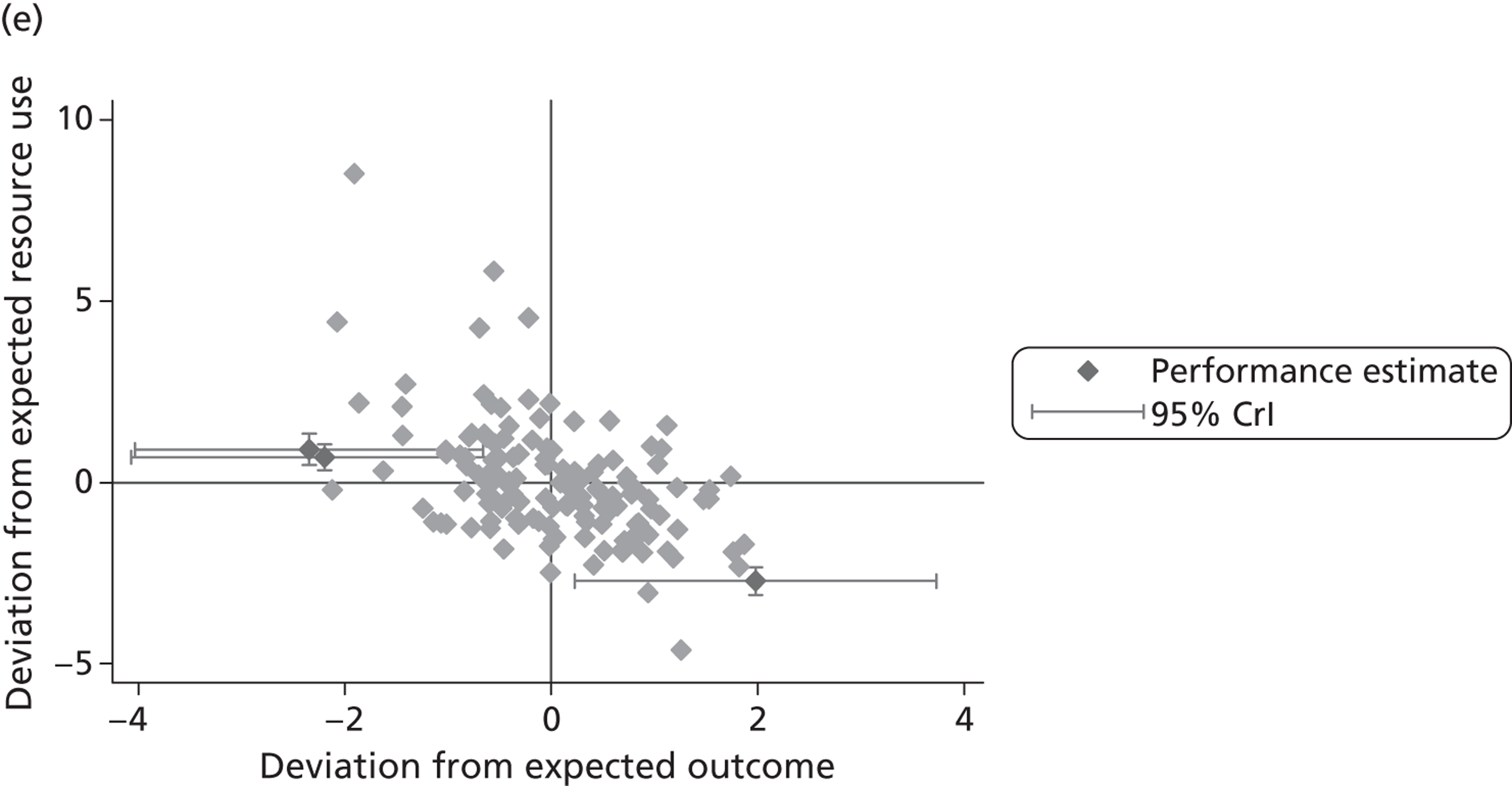
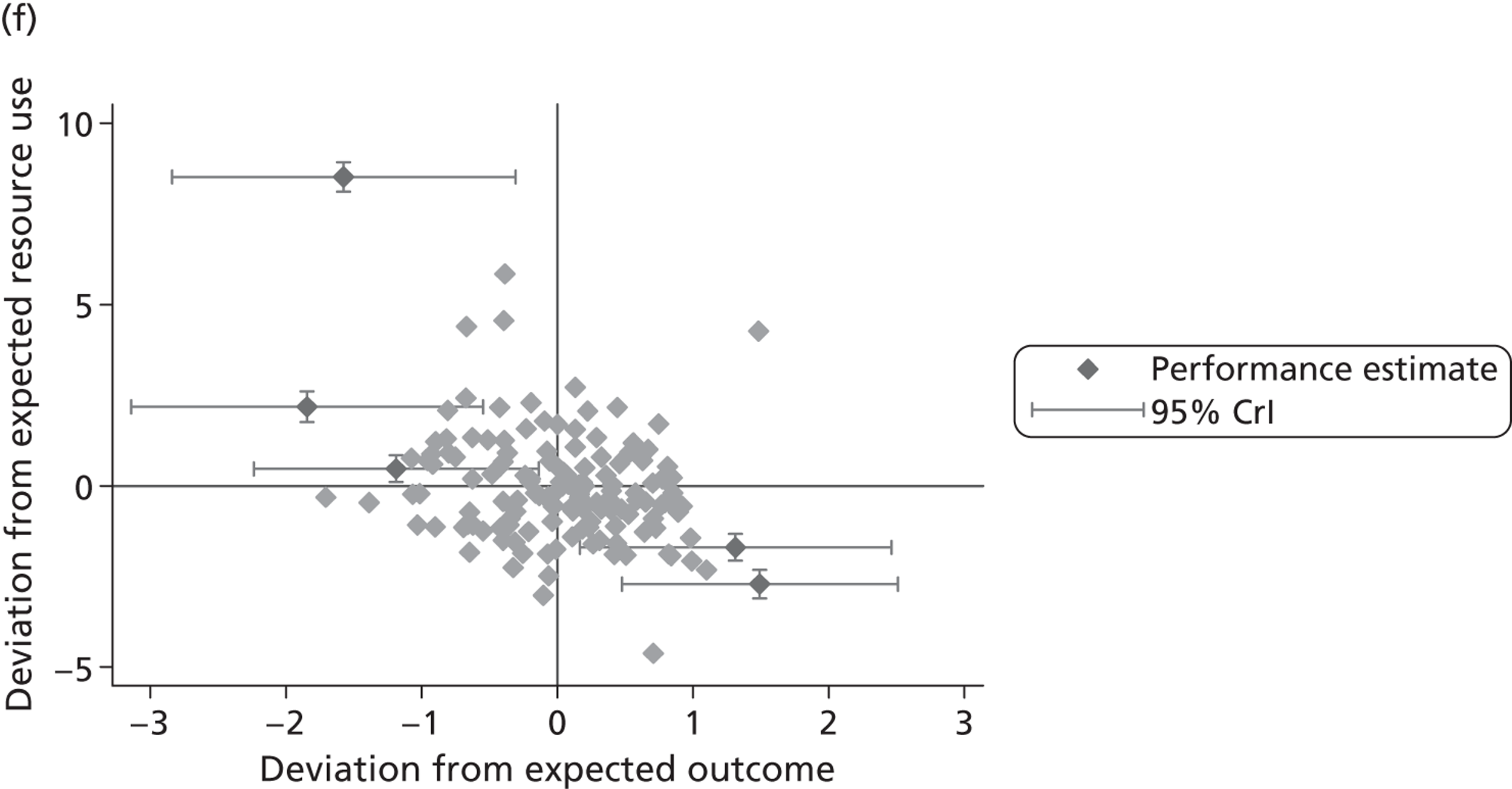
FIGURE 22.
Joint cost and quality performance estimates – knee replacement. (a) LoS/EQ-5D index; (b) LoS/EQ-VAS; (c) LoS/OKS; (d) cost of treatment/EQ-5D index; (e) cost of treatment/EQ-VAS; and (f) cost of treatment/OKS.
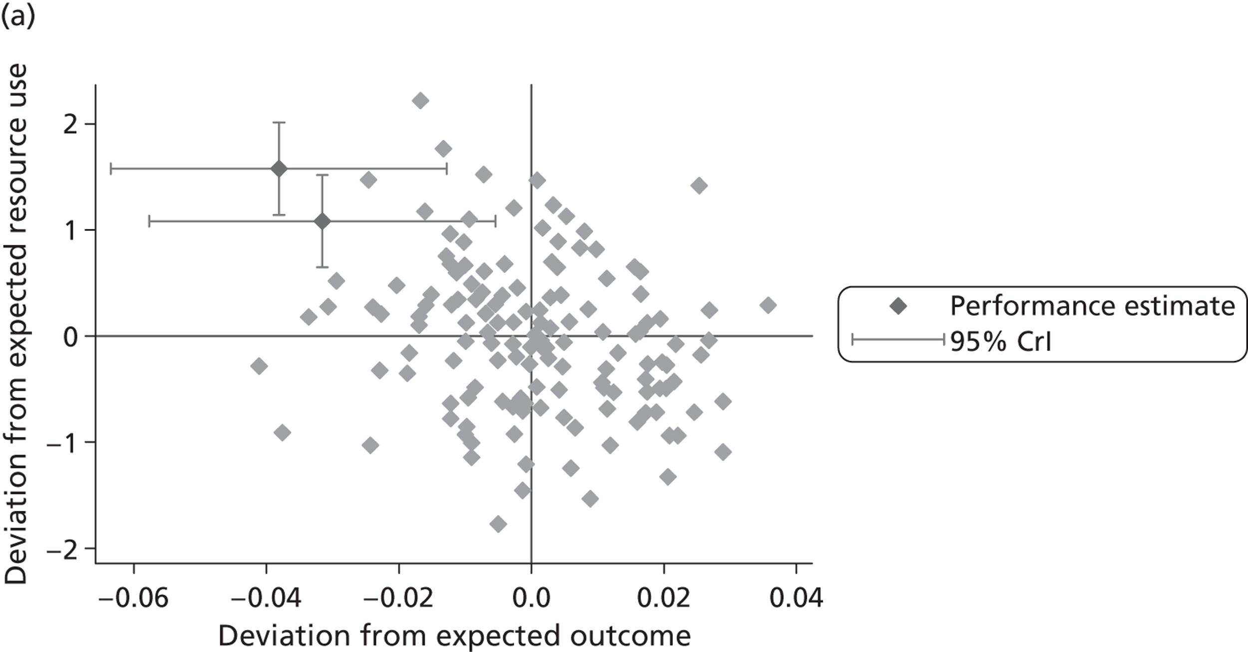
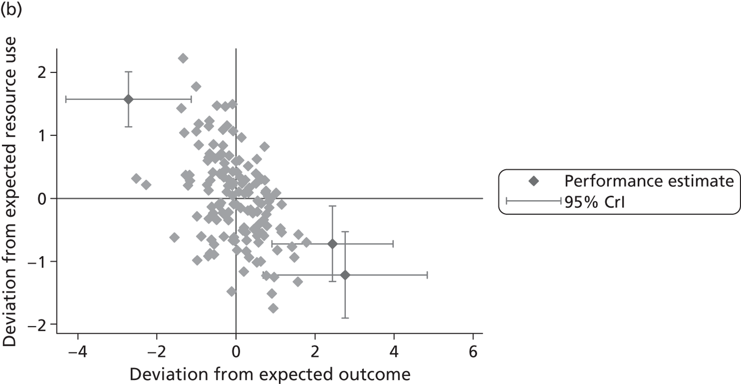
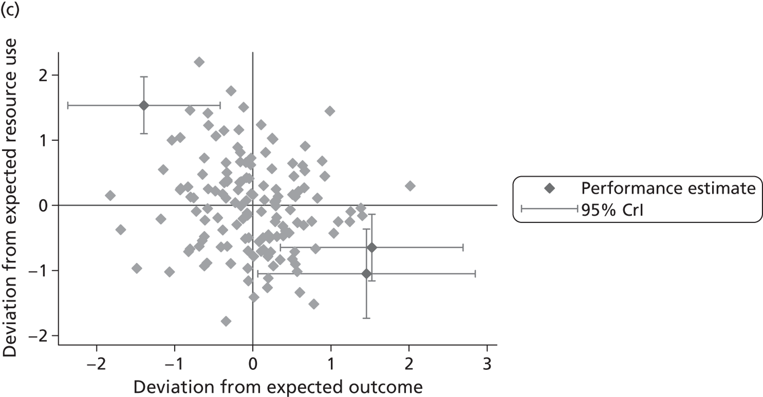
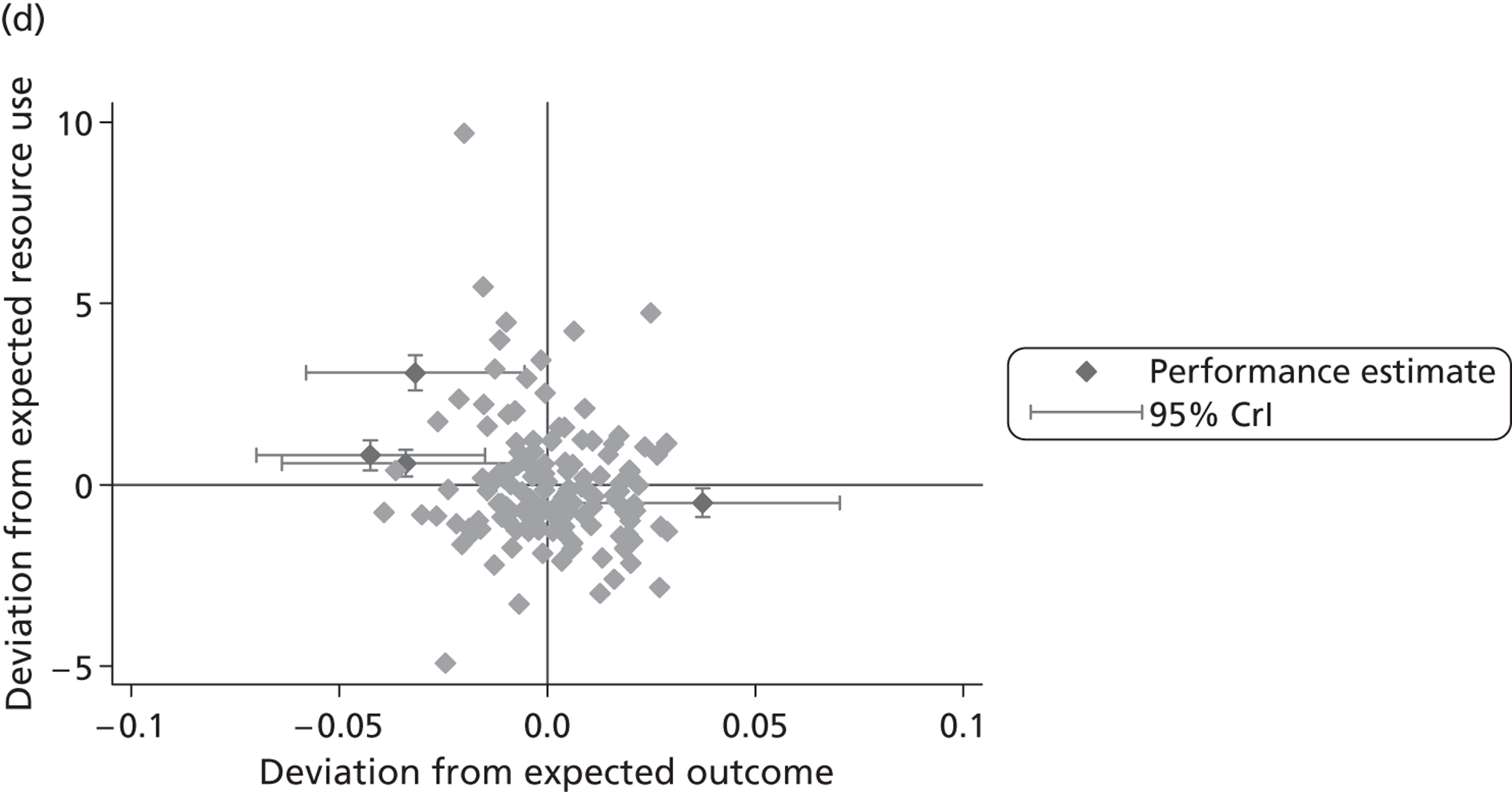
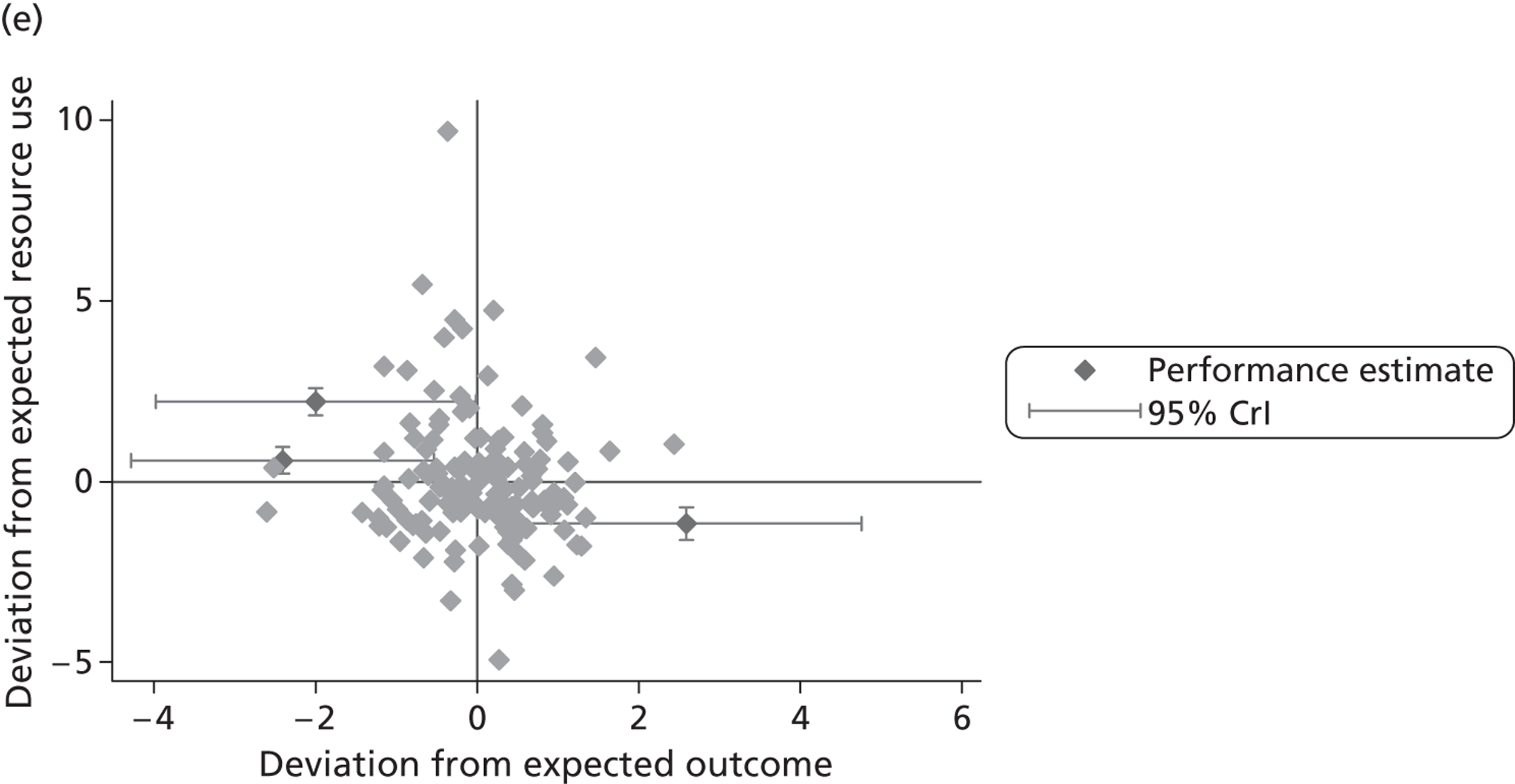
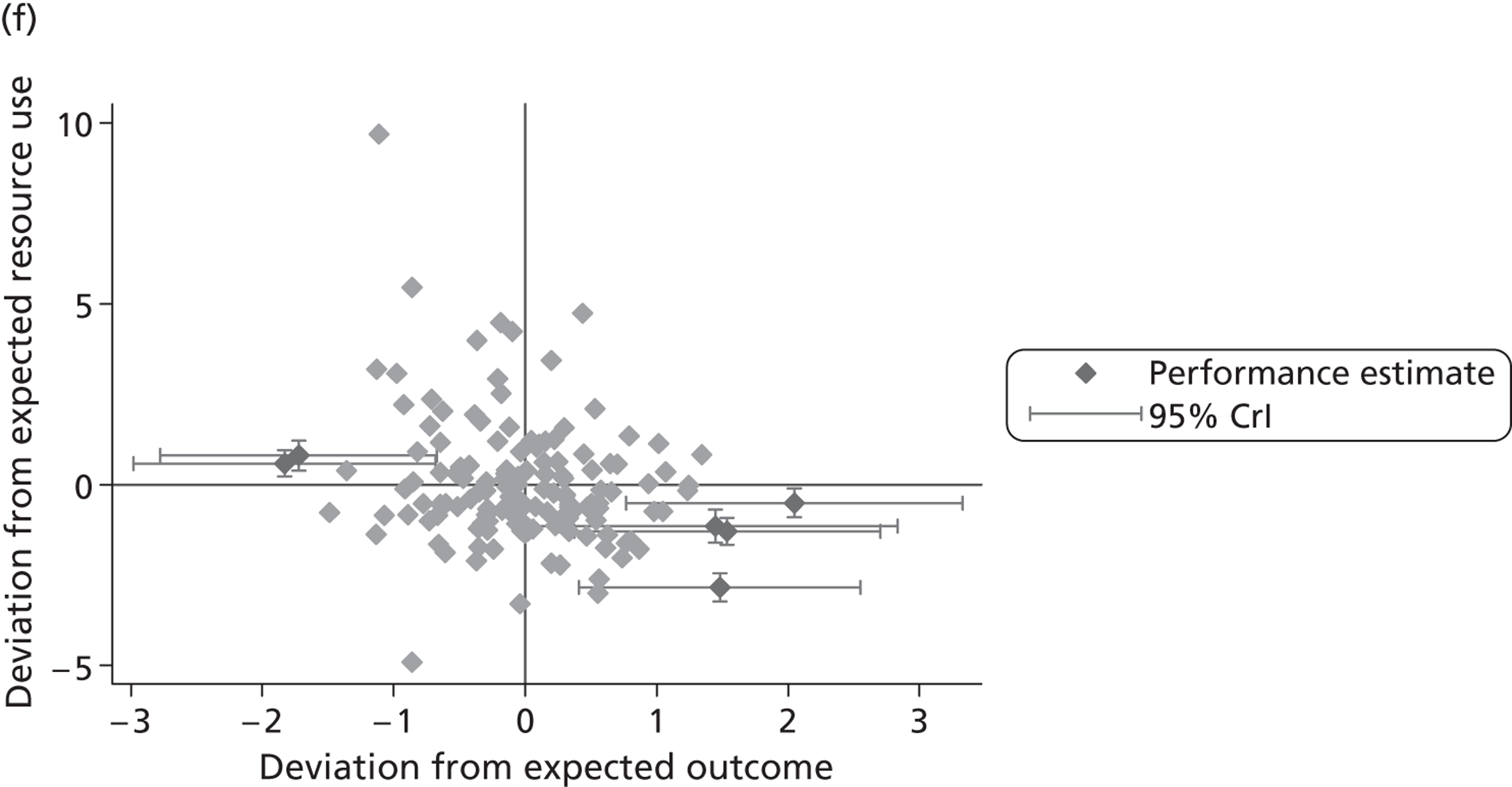
The effect of risk adjustment
Figures 23 and 24 illustrate the impact that risk adjustment has on the conclusions to be drawn at hospital level regarding the relationship between outcomes (plotted on the x-axis) and resource use (plotted on the y-axis) for hip replacement ( Figure 23 ) and knee replacement ( Figure 24 ). The grey dots indicate each hospital’s relative performance in terms of the average outcomes and resource use for its patients when no risk adjustment is undertaken. The black crosses indicate each hospital’s relative performance after accounting for the influence of patient and hospital characteristics.
FIGURE 23.
Effect of risk adjustment on joint resource use and health outcome performance – hip replacement. (a) LoS/EQ-5D index; (b) LoS/EQ-VAS; (c) LoS/OHS; (d) cost of treatment/EQ-5D index; (e) cost of treatment/EQ-VAS; and (f) cost of treatment/OHS.
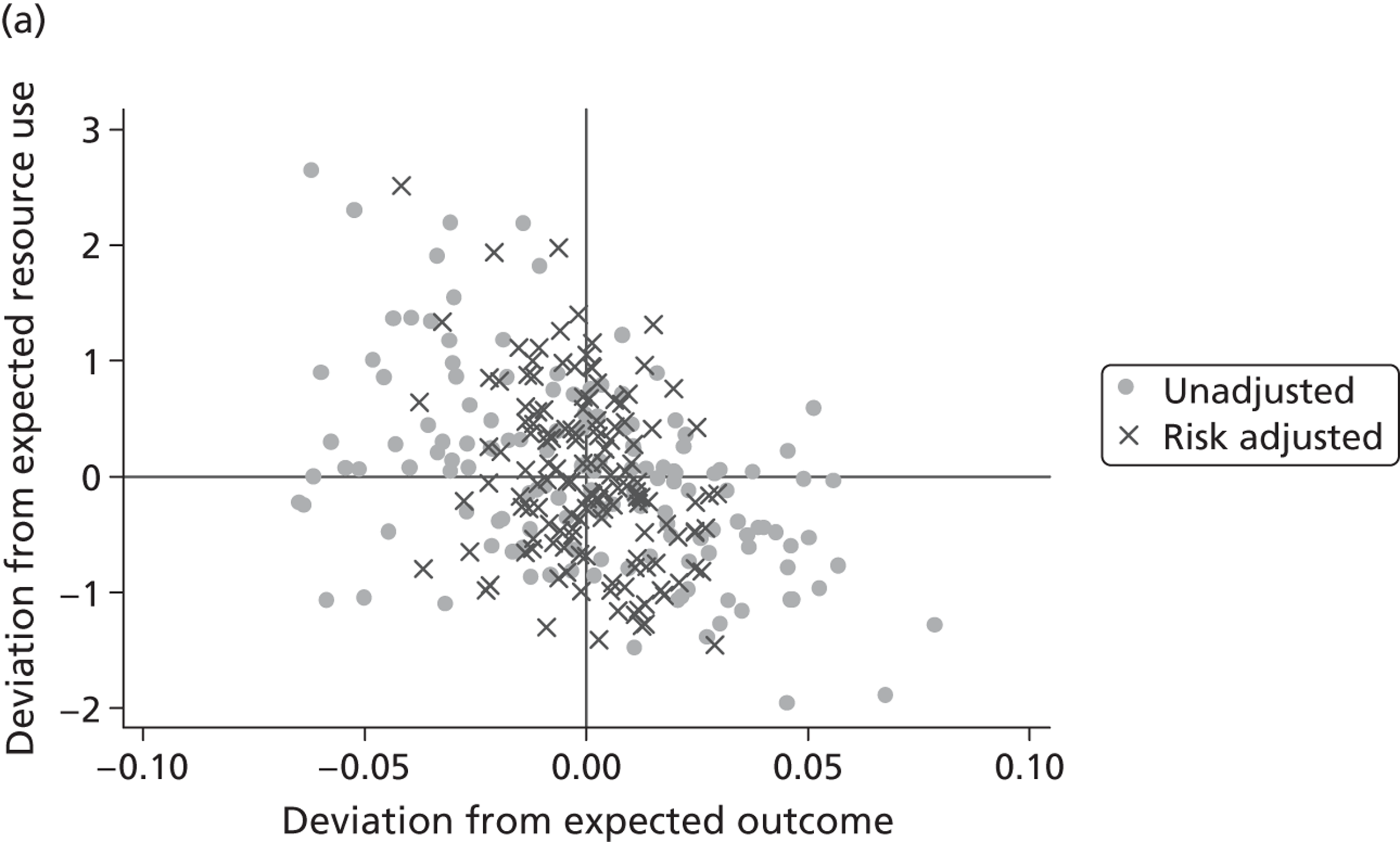
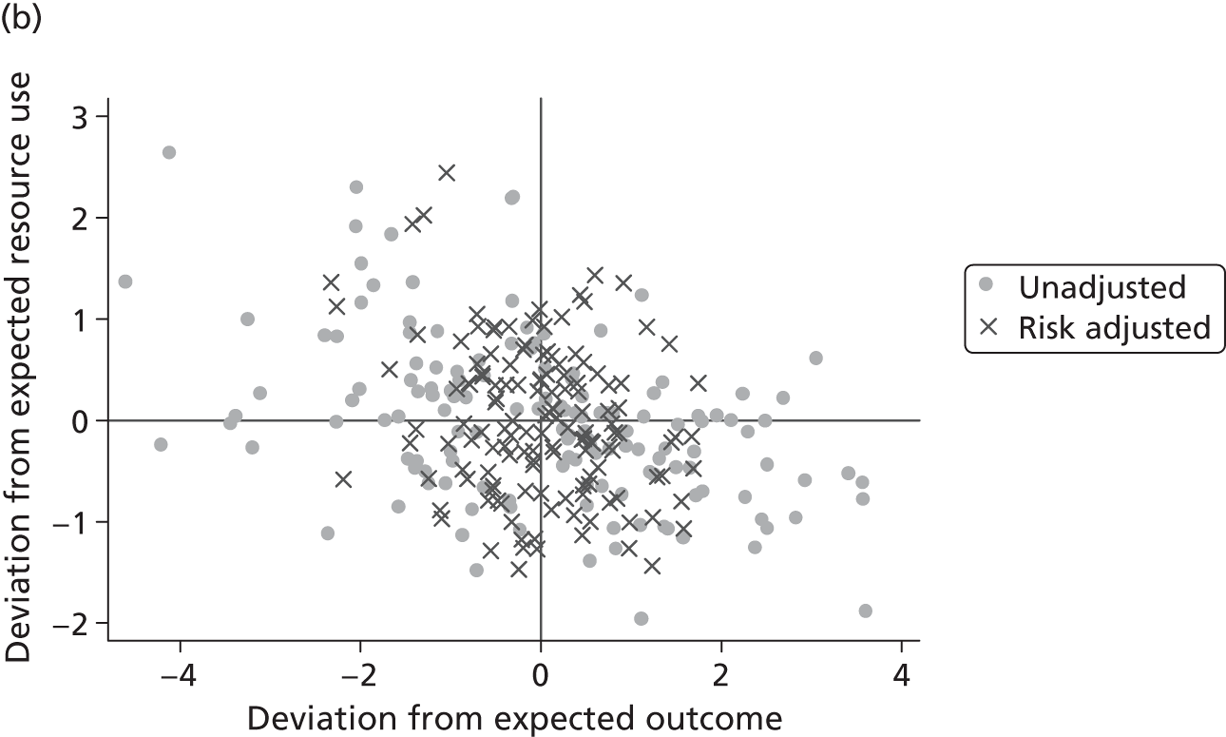
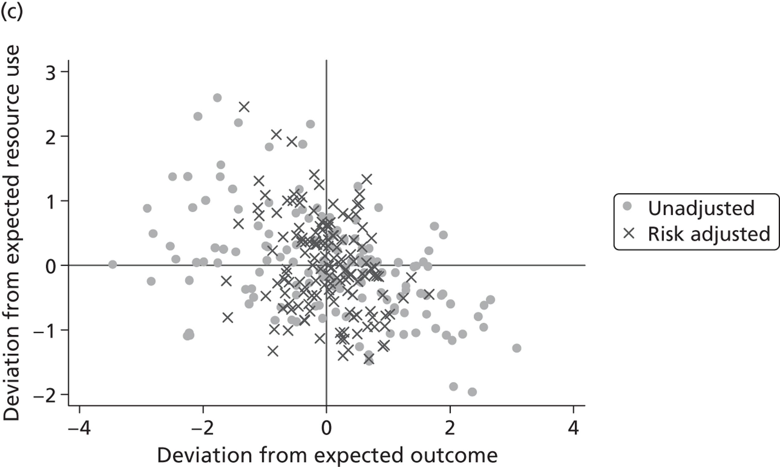
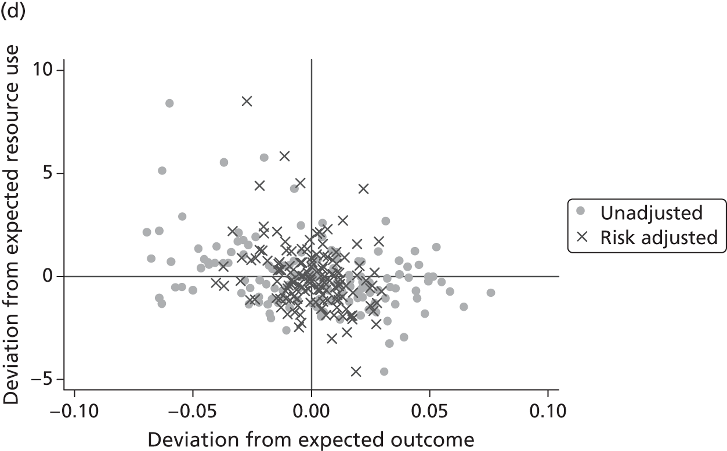
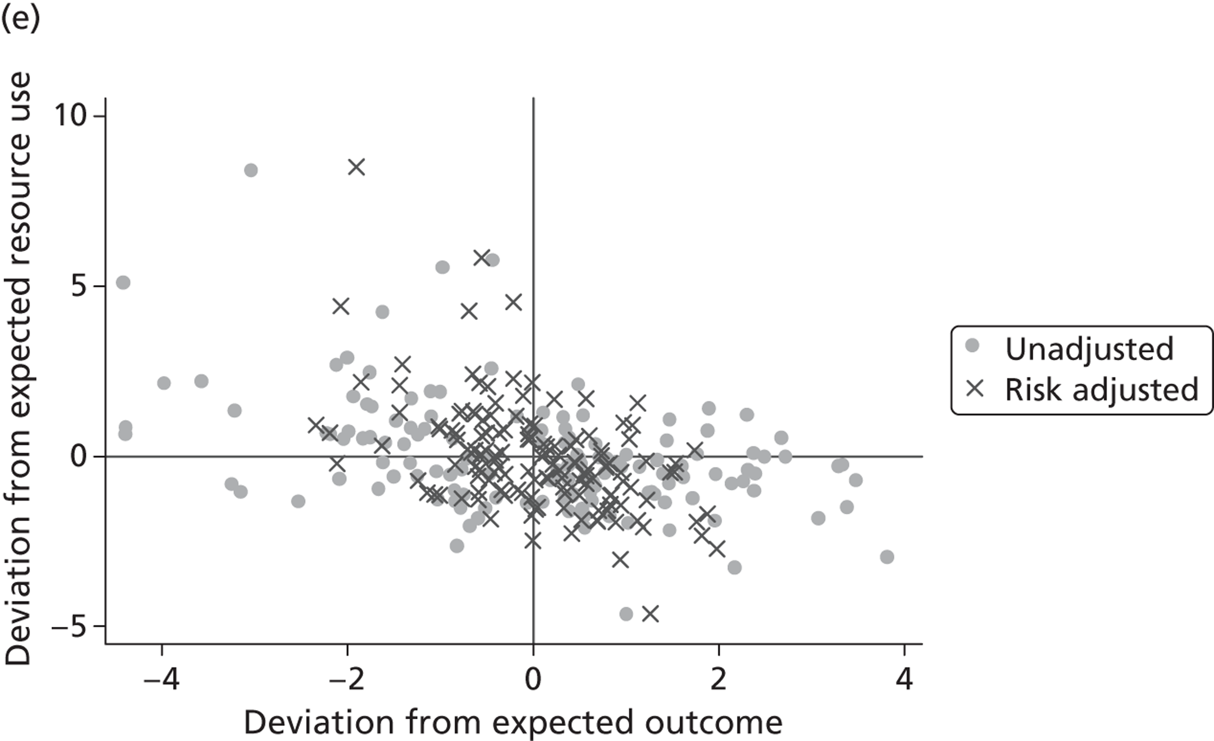
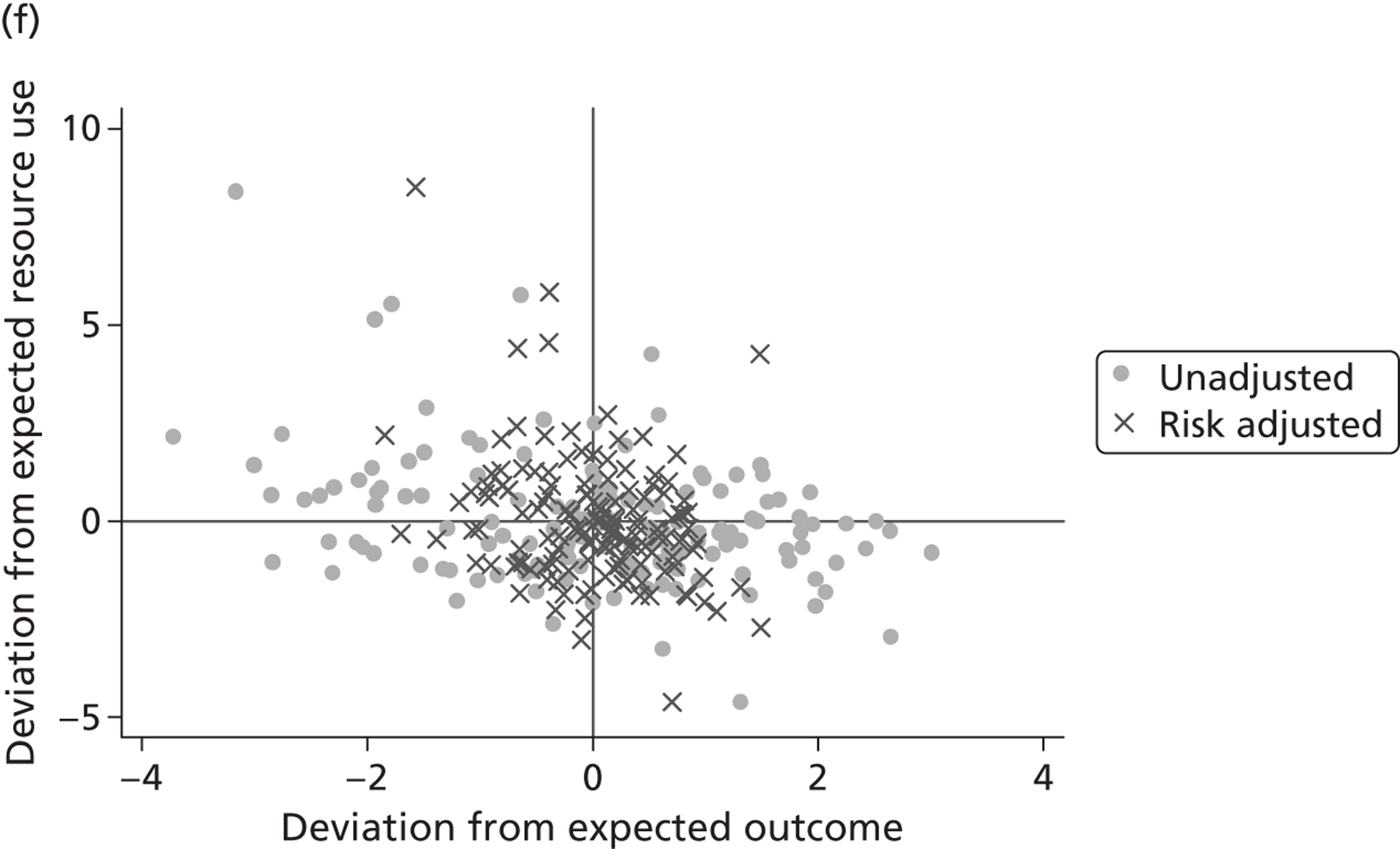
FIGURE 24.
Effect of risk adjustment on joint resource use and health outcome performance – knee replacement. (a) LoS/EQ-5D index; (b) LoS/EQ-VAS; (c) LoS/OKS; (d) cost of treatment/EQ-5D index; (e) cost of treatment/EQ-VAS; and (f) cost of treatment/OKS.
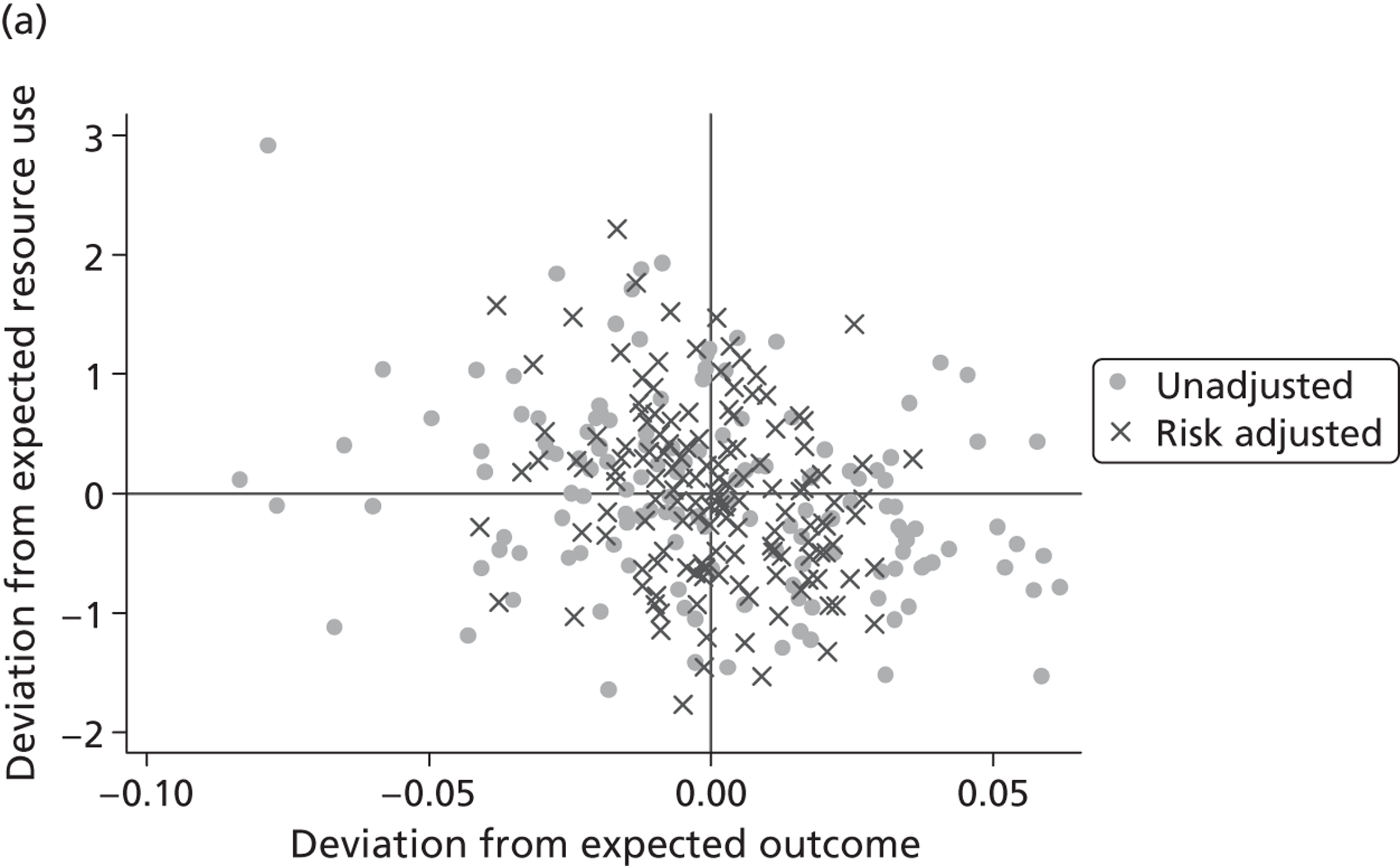
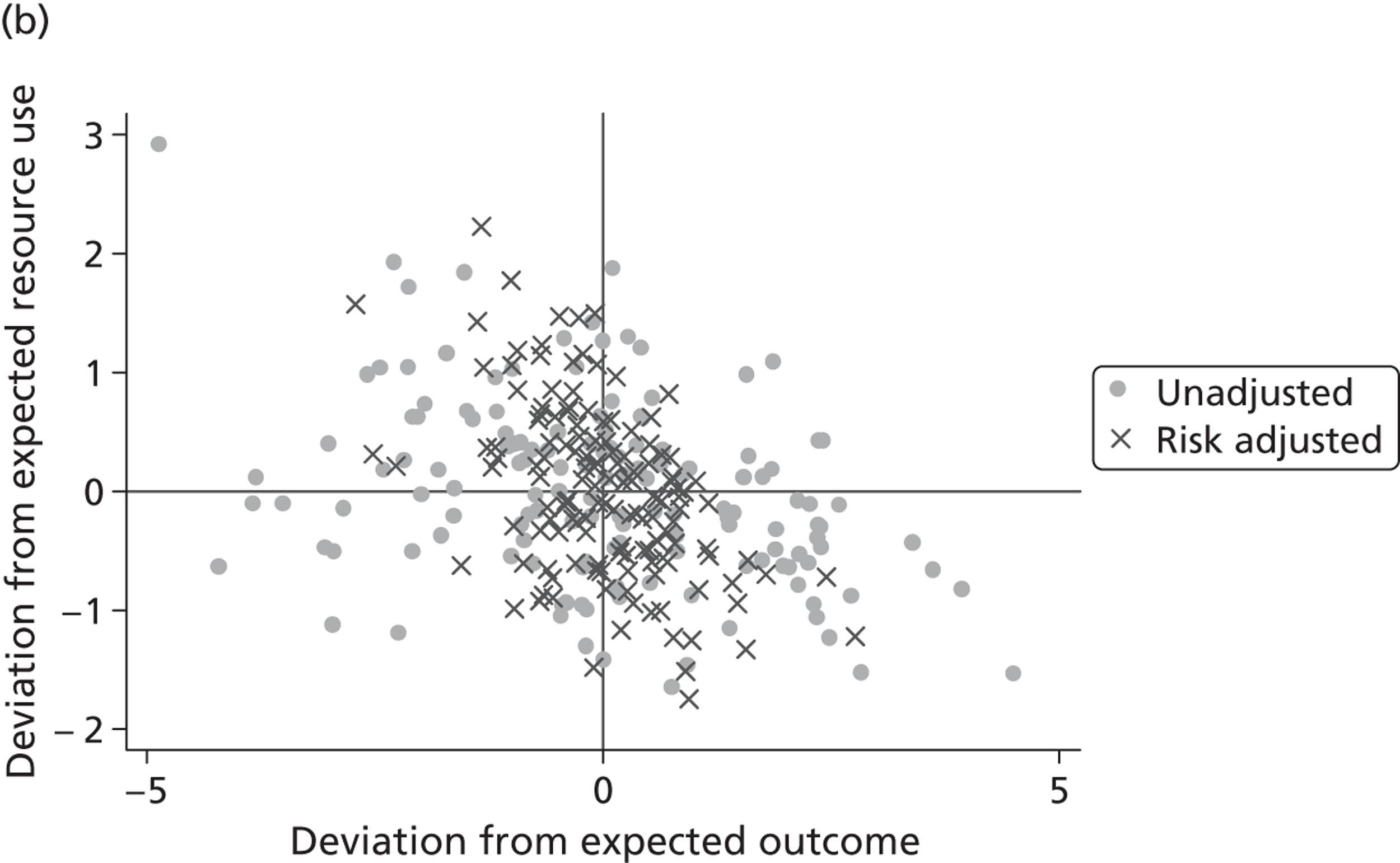
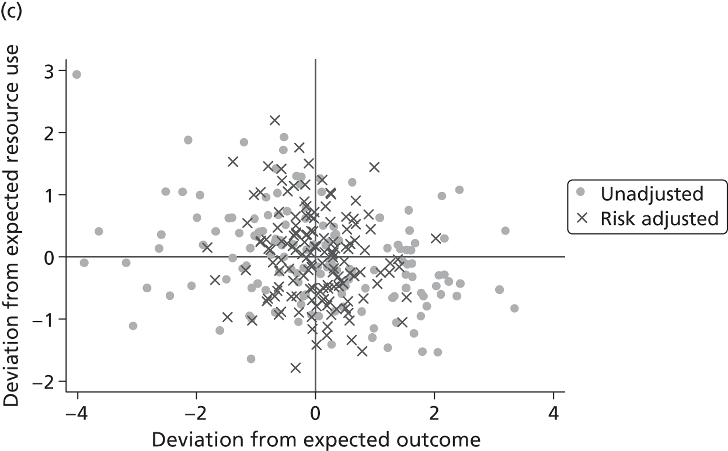
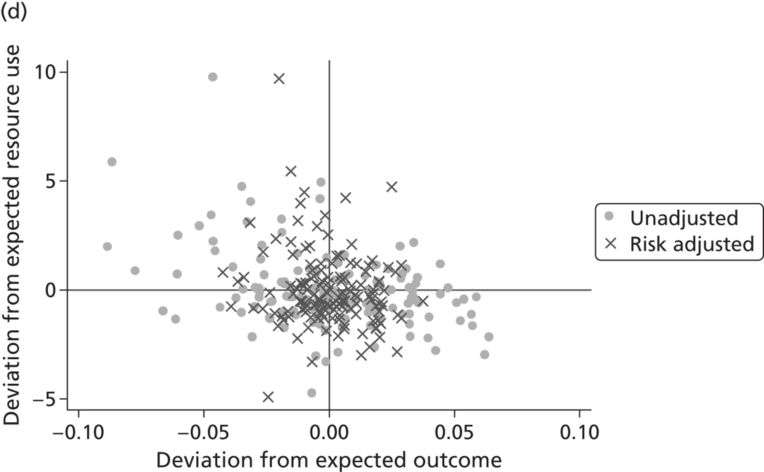
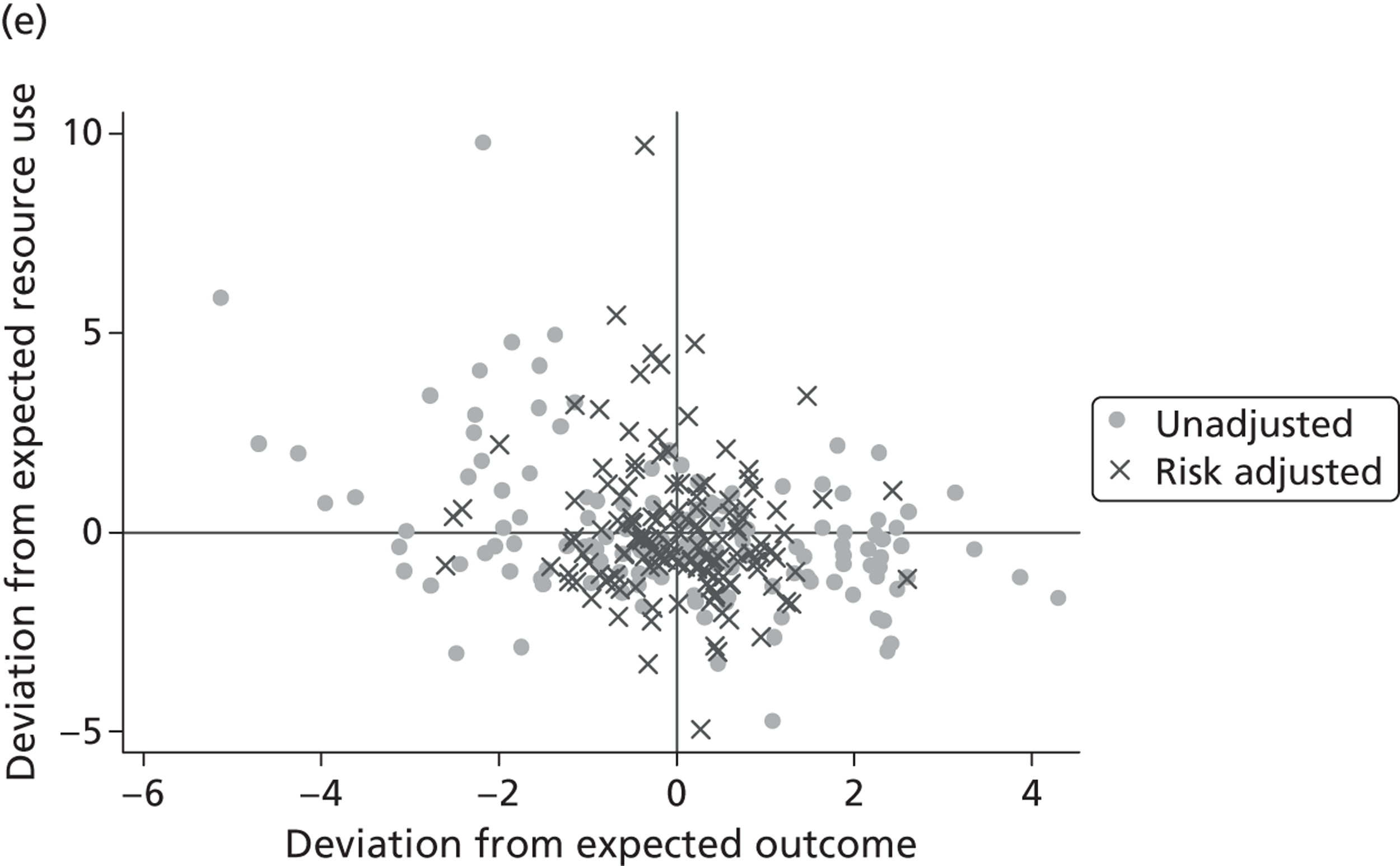
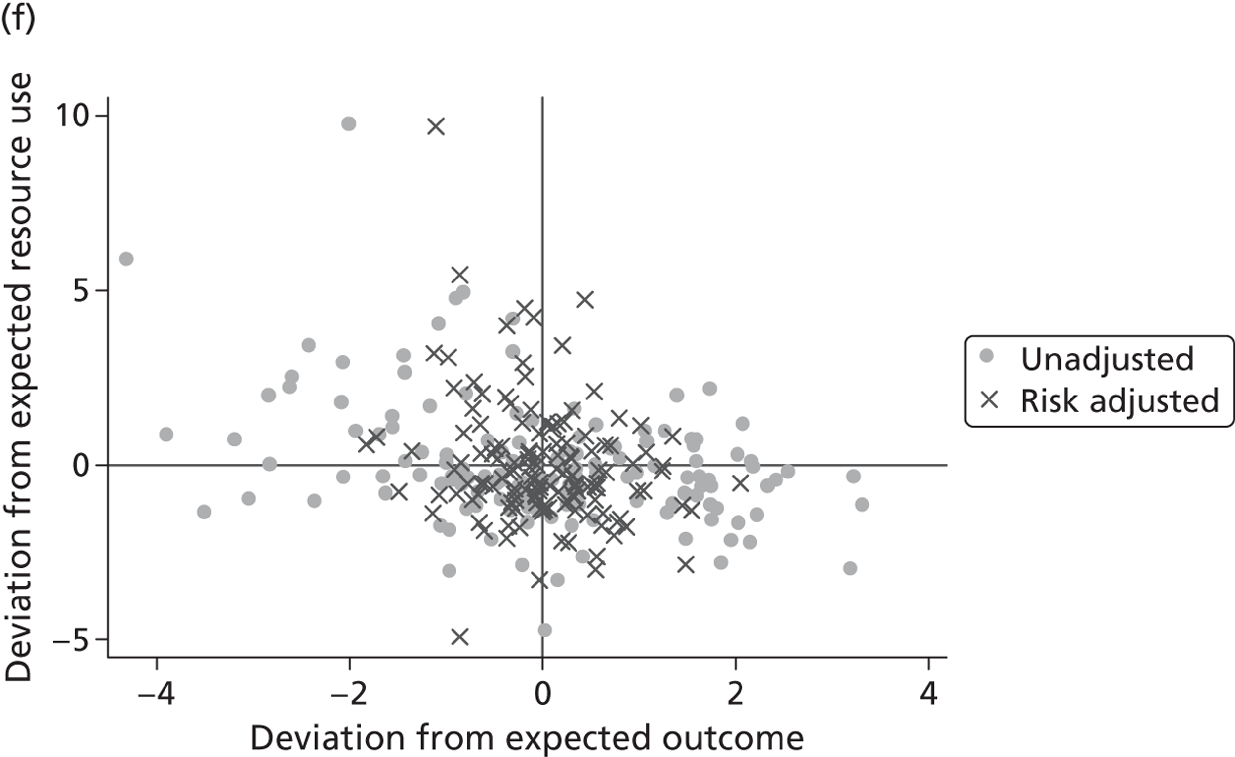
The most noticeable impact is on the estimation of hospital effects on outcomes, regardless of the PROM considered. The distribution of effects is substantially narrower when we adjust for patient case mix and production constraints than when we do not risk adjust. In contrast, the estimates of hospital effects relating to resource use show little sign of adjustment, as reflected in the approximately equal dispersion of effects before and after adjustment for case mix and production constraints. For outcomes, this suggests that not only is there an uneven distribution of patient case mix across hospitals but also that observable characteristics explain a significant amount of the variation that we observe in the unadjusted measures. For resource use, the observable characteristics of patients do not explain a great deal of observed variation. One reason for this may be that for outcomes, the before-and-after nature of data collection provides a very good opportunity to identify variations among patients beyond that which is systematically related to other observable characteristics, such as age. In other words, our ability to risk-adjust is greatly improved by having information on pretreatment health status and the impact of this is clear in the narrowing of the distribution. This does raise issues for the reliability of risk adjustment in other, more traditional, areas of performance measurement, e.g. standardised mortality rates or readmissions. Although the pretreatment PROM score was used as an explanatory variable in the resource use equations and does indeed explain some of the variation in resource use, the impact of risk adjustment is markedly less pronounced.
Chapter 5 Discussion
The routine collection of PRO data is long overdue and this English exercise promises to be an important component of international efforts to improve health-care provision. In this project we set out to (1) characterise variation in outcomes in ways that are intuitive to patients and consistent with the original format of the questionnaire, thereby helping them select a preferred provider of care and (2) assess the relationship between the cost and outcomes of the four elective procedures for which PROMs data are collected and to determine the extent to which variations in outcome and cost ratios are due to differences in hospital performance.
To meet the first aim, we measure variability in hospital quality in hip replacement surgery, which necessitated meeting a number of methodological issues. Most previous efforts have focused on ensuring adequate risk adjustment; however, our paper focuses on three methodological issues that have received less attention to date.
First, rather than focusing on an aggregate PROM score, we argue that it is both more accurate and more informative to assess each of the PROM dimensions in their own right. Our approach does not require assumptions to be made regarding how to aggregate across health dimensions and offers insight about which dimensions are particularly affected by hospitals. We set out an analytical strategy to explore patient- and hospital-level variation in categorical responses within and across dimensions of the EQ-5D. We find variation in performance to be more pronounced across the mobility and usual activities dimensions. In contrast, the performance on the pain/discomfort, anxiety/depression and self-care dimensions is less varied. These insights cannot be gained from the EQ-5D utility data and, furthermore, we find that performance on the utility scale correlates well only with the anxiety/depression and pain/discomfort dimensions. Incidentally, these are the dimensions that receive the highest weighting in the UK EQ-5D tariff. 11 In contrast, the dimensions mobility, usual activities and self-care have relatively low weights attached to them and variation in performance across hospitals remains undetected when analysing aggregate EQ-5D data.
Second, policy interest is in assessing the change in patient-reported health status as a result of treatment. There are various ways that this change can be measured and modelled. Our approach has been to model both pre- and post-treatment health status as resulting from the same reporting process and to conduct multilevel analysis with measurement points clustered in patients, which themselves are nested in hospitals. We argue that this is the appropriate modelling strategy because it acknowledges the features of the data-generating process, allows for patient heterogeneity, with respect to observed and unobserved factors, and makes best use of the available information. The presented methodology is readily applicable to other conditions for which the EQ-5D data are collected and can also, in principle, be extended to other instruments.
Third, in recognition of the expectation that health outcome data are to be used by an audience unfamiliar with the interpretation of complex statistical results (e.g. patients and their relatives, purchasers of care and family doctors), we have suggested an intuitively appealing and accessible way of summarising the differential impact that hospitals have on treatment outcomes. Our graphical representation indicates the probability of reporting a given health outcome and shows how these probabilities vary across health dimensions and hospital providers. Prospective patients who place greater weight on one or more particular dimension may use this information to select a hospital that has a differentially greater impact than its peers do. Health-care providers should engage in clinical audits to identify the reason for variation.
The primary limitation of our proposed approach is the increase in dimensionality of the decision problem for patients. Where aggregated scores result in one estimate of hospital performance, our approach generates five, potentially divergent, answers. In a recent study, Dijs-Elsinga et al. 65 have shown that a large group of patients favour simple data presentation and prefer one overall measure of hospital quality; however, many patients intend to use more detailed quality information when making decisions about where to seek care in the future. 65 The question then arises of how much information should be provided for the different objectives for which performance information can be used (i.e. patient choice, accountability, identification of best practice) and who decides the relative weighting of each component and objective. 12,66 Our study does not intend to resolve this debate. Rather, we present a means of making inferences about hospital quality and presenting results when health outcomes are assessed through the EQ-5D instrument. How best to communicate such performance data requires careful consideration, to ensure it can be effectively understood and used.
Our second aim has been to investigate the relationship between hospital-level measures of health outcome and resource use after allowing for patient case mix and hospital caseload. We do this by constructing multilevel health outcome and resource use equations using data from individual patients treated for one of four elective procedures in the English NHS. By formulating the regression models of resource use and outcomes as a system of equations estimated in a SUR framework, we are able to gain additional insight into the correlation between unobserved factors that drive both resource use and outcomes.
In keeping with the wider literature, we find that the observed patient characteristics conform to a priori expectations in the manner that they affect resource use and outcomes across all four conditions. As expected, we find significant unexplained interpatient variation in resource utilisation and outcomes after allowing for observed characteristics. We also find that for all four conditions there is significant unexplained variation in resource use among hospitals, whether this is measured by cost of treatment or LoS. There is also unexplained variation among hospitals in the health outcomes experienced by patients having hip replacement, knee replacement or varicose vein surgery. These results suggest room for improvement among hospitals in both their utilisation of resources and patient outcomes. In contrast, there is no substantial variation among hospitals in outcomes for groin hernia patients, rendering the information redundant for benchmarking hospital performance for these patients.
One of the novelties of this aspect of the work is the use of correlated error terms across equations at patient and hospital levels. As expected, at the patient level we find a negative correlation between resource use and outcomes for hip replacement and knee replacement. This suggests that, despite the detailed nature of the observed characteristics, including the pretreatment level of health, omitted factors exist that drive both resource use and health improvement in opposite directions.
However, we find no significant general correlation between resource use and outcomes at hospital level across all four conditions. Plots of the hospital-specific effects for both resource use and outcomes confirm this conclusion with, for many of the PROM and resource use combinations tested, the general mass of points looking randomly distributed without any obvious systematic relationship. In the cases where we identify a systematic relationship, this tends to be negative. This would suggest that overall there is scope to improve technical efficiency in the provision of elective surgery. Some hospitals could achieve better outcomes by learning from other, best practice hospitals, without increasing costs; similarly, other providers could reduce costs without compromising, or even by improving, health outcomes.
Very few hospitals are identified as positive or negative outliers; however, there are a few instances of high-cost or -quality hospitals that could potentially justify the extra average costs of their procedures by noting that the outcomes reported by their patients are better than expected. Whether or not the gain in health outcomes is worth the additional cost and is, therefore, optimal for the NHS {i.e. below a NICE-style cost per quality-adjusted HES [QALY; (quality-adjusted life-year) threshold]} is difficult to tell given the absence of sufficient follow-up data to calculate QALYs.
Implications for practice
This study has the following implications for practice:
-
Choice of instrument. The EQ-5D and condition-specific measures tend to broadly agree in that they show the same general properties in terms of post-treatment improvements. However, the PRO measures do not always identify the same number of hospitals as outliers. The EQ-VAS, in contrast, shows counterintuitive results in terms of increased post-treatment distributions and an overall negative change for groin hernia treatments. We believe that this implies that the EQ-VAS may be subject to greater error than the other two measures. Given that the generic EQ-5D measure may be used across conditions and produces results that are generally in accordance with the condition-specific measures, and that the EQ-VAS seems a noisier generic measure with no greater sensitivity, we can find little to recommend the continued use of the EQ-VAS as a PROM. Indeed, since we commenced our study, the Department of Health has decided that collection of EQ-VAS data is no longer required as part of the PROM survey.
-
Presentation of PROMs information to prospective patients. Careful consideration should be given to the way in which PROM information is presented to patients and other stakeholders. PROM scores, such as utility scores represented by the EQ-5D index, are not readily understood, or easily interpreted, by a non-technical audience. Instead, hospital providers and the NHS Information Centre should work towards translating results into more intuitive metrics, such as percentages, and present results on the same scale on which PROM responses are provided. Our graphical presentation of the probability of reporting a specific post-treatment health status category is an example of how to do this.
-
Incentivise providers to improve participation rates. We find that, in our dataset, only 40.6% of eligible hip replacement patients participate in the baseline survey and provided a complete EQ-5D health profile, with a further 8% dropping out of the subsequent survey (see Missing data). The best solution to dealing with missing data is to improve response rates. This is happening. Hospitals are increasing the proportion of patients who undertake the survey by making the data collection procedures more effective. 67 Further efforts are required to maintain this momentum and achieve consistently high participation rates over time, thereby reducing the risk that inferences about performance are based on incomplete and potentially unrepresentative data.
-
Learn from good practice and challenge poor performance. Our analysis sorts hospitals into four quadrants according to their performance in relation to both their costs and outcomes, having controlled for case mix and hospital characteristics. A handful of hospitals in the south-east quadrant perform significantly better than the national average and some hospitals in the north-west quadrant perform significantly worse than the national average. The question is what may drive their better (or worse) performance in relation to the procedure in question. The reasons may be due to differences in coding practices, working relationships, staff mix, theatre and ward layouts, organisational culture, etc. None of these reasons are observable from routine data and identification requires site visits and qualitative study. Our analysis identifies which of the English NHS hospitals merit a visit and what types of activity the visit should focus on, such as those caring for patients having the particular procedure.
-
Measure and evaluate PROMs for other hospital conditions. The PROMs initiative focused initially on the four common surgical procedures evaluated in this report. These represent only 1.6% of total hospital activity. To gain a fuller picture of hospital performance, PROMs should be extended to other areas of hospital activity. This should first be rolled out to those conditions or procedures where existing evidence suggests wide variation in costs and/or other measures of quality.
-
It may be unnecessary to introduce a PROMs premium/penalty for these procedures under payment by results. The Department of Health has raised the possibility of making payments based on PROMs, a suggestion which has met with some resistance. 68 Our research suggests PROM-related payments are probably a blunt instrument – only a handful of hospitals have significantly better (or worse) PROMs than the national average so, by implication, only a few would be affected by differential rewards. Furthermore, for hip replacement or knee replacement, we found a negative association between cost of treatment and outcome, so better performance with respect to outcomes does not seem to require higher resource inputs. For these procedures, mechanisms other than pay-for-performance may be more effective at reducing variation in performance.
Implications for research
Several issues remain that we have not addressed in this study that have implications for future research.
-
Improve methods to deal with missing data. The problem of missing data pervades all research. Based on the full information contained in HES, we can identify those patients who have not participated or were not included in the follow-up. Falsely assuming that any substantial number of missing values are generated at random could lead to biased inferences from a non-representative population,43,44 raising questions regarding the validity of the assessment. Efforts are currently being made to identify the reason for non-response. 69 Given that it will be impossible to eradicate completely the problem of missing data, future research should be directed towards developing methods for handling missing data in the specific setting discussed here. Current methods, such as standard multiple imputation, may be a valuable starting point; however, these methods may not be directly transferable to hierarchical and non-randomised settings, such as characterised by the PROMs data.
-
Collect data that characterise patient severity. In this study we have controlled for patient risk factors that are deemed clinically relevant, assumed to be exogenous to the hospital and can be derived from routine inpatient records. However, we do not claim that this set of control variables is exhaustive. Health outcomes may be affected by non-randomly distributed and unobserved patient characteristics, such as severity of the medical condition or health-related behaviour. However, a key strength of our study is that we control for the pretreatment health status. We believe that the health status with which the patient presents prior to treatment contains much information to mitigate any bias resulting from unobserved severity, making our analysis more robust than otherwise possible. In many studies, pretreatment health status is unobserved.
-
Evaluate hospital performance in the context of the broader health economy. Throughout this study we have assumed that, after controlling for a wider array of patient characteristics, the remaining variation in changes in reported health can be interpreted as a result of variation in hospital quality. This is the common interpretation given to risk-adjusted outcome measures such as readmission or 30-day mortality rates. But hospitals are but one part of the care pathway. For instance, procedures such as hip replacement are generally followed by extensive physiotherapy and these services are often delivered outside the hospital environment and variation in quality may not be attributable solely to the hospital of inpatient care. Further work is required to ascertain what pathway-related care is provided subsequent to hospital discharge and to establish the sensitivity of hospital quality assessments to this provision.
-
Incorporate PROMs in the broader quality assurance framework. Further consideration should be given to the role that PRO performance information can play in the existing quality assessment framework. While measures of risk-adjusted mortality, readmission and adverse events have been criticised for their limited granularity and sensitivity,70 one should not dismiss their ability to identify high- and low-quality providers of care. Further research is required to establish the additional value of outcome data for hospital quality assessments and contrast it to the costs of collection.
-
Investigate means of communicating information about variations in hospital PROM performance to patients. PROMs are new measures that have the potential to help patients assess hospital quality. For example, in contrast to mortality rates, PROMs do not have a straightforward and well-understood interpretation. 16 Further research is required into how best to ensure consistency between the analytical approach and dissemination of results to a relevant audience. For example, our suggested way of presenting cumulative proportions of EQ-5D dimensions merits qualitative research into its acceptability and interpretability.
-
Evaluate the impact of the PROMs initiative on patient choice and provider behaviour. The introduction of PROMs was motivated partly to inform patients about where to seek care and to encourage hospitals to scrutinise and improve the quality of their care. Have these motivations been realised? The evidence is not yet available. A before-and-after longitudinal study that controls for other contemporaneous influences would be required to isolate the impact of PROMs on patient and provider behaviour. As more data become available, such a study should be feasible.
-
Measure and evaluate PROMs for chronic conditions. The PROMs initiative is being considered for people suffering from long-term conditions such as asthma, diabetes mellitus and heart failure. This presents novel methodological challenges because (1) the purpose of care may not be curative but rather to arrest the speed of decline of the condition, (2) care is usually delivered over extended time periods and (3) patients may receive multiple types of intervention delivered by different hospitals. Research is required to address these challenges and to evaluate the impact of care on the health of the large group of the population that lives with chronic conditions.
Acknowledgements
We would like to thank Stephen Barasi, Stephen Bloomer, Stirling Bryan, Wolfgang Greiner, David Nuttall, David Parkin and Aurore Pelissier, as well as participants of the Health Econometric Data Group seminar series (York), the EuroQoL plenary meeting 2012 (Rotterdam), the joint CES-HESG Winter conference 2012 (Marseille) and the HESG Summer conference 2012 (Oxford) for their valuable inputs and comments. The views expressed are those of the authors and may not reflect those of the NIHR HSR programme or the Department of Health.
Findings from the first part of the work are to be published as:
Gutacker N, Bojke C, Daidone S, Devlin N, Street A. Hospital variation in patient-reported outcomes at the level of EQ-5D dimensions - Evidence from England. Med Decis Making 2013 33(6):804–18. doi:10.1177/0272989X13482523.
Contributions of authors
Andrew Street (Professor, Health Economics) was responsible for the overall management and delivery of the project.
Nils Gutacker (Research Fellow, Health Economics) was responsible for data management and manipulation, and for execution of the econometric analyses.
Chris Bojke (Senior Research Fellow, Health Economics) was responsible for the day-to-day management of the project and provided statistical expertise.
Nancy Devlin (Professor, Health Economics) provided leadership on the analysis of the PROMs data and comparison of instruments.
Silvio Daidone (Research Fellow, Health Economics) provided guidance on the empirical analysis of cost and PROM data.
Disclaimers
This report presents independent research funded by the National Institute for Health Research (NIHR). The views and opinions expressed by authors in this publication are those of the authors and do not necessarily reflect those of the NHS, the NIHR, NETSCC, the HS&DR programme or the Department of Health. If there are verbatim quotations included in this publication the views and opinions expressed by the interviewees are those of the interviewees and do not necessarily reflect those of the authors, those of the NHS, the NIHR, NETSCC, the HS&DR programme or the Department of Health.
Publications
Gutacker N, Bojke C, Daidone S, Devlin N, Street A. Analysing hospital variation in health outcome at the level of EQ-5D dimensions. Centre for Health Economics, CHE Research Paper 74. York: Centre for Health Economics, University of York; 2012.
Gutacker N, Bojke C, Daidone S, Devlin N, Street A. Hospital variation in patient-reported outcomes at the level of EQ-5D dimensions - Evidence from England. Med Decis Making 2013 33(6):804–18. doi:10.1177/0272989X13482523.
References
- Appleby J, Devlin N. Measuring Success in the NHS: Using Patient Assessed Health Outcomes to Manage the Performance of Health Care Providers. London: Dr Foster; 2004.
- Guidance on the Routine Collection of Patient Reported Outcome Measures (PROMs). London: The Stationery Office; 2008.
- Holmstrom B, Milgrom P. Multi-task principle-agent problems: incentive contracts, asset ownership and job design. J Law Econ Org 1991;7:24-52.
- Shleifer A. A theory of yardstick competition. RAND J Econ 1985;16:319-27. http://dx.doi.org/10.2307/2555560.
- Iezzoni L. Risk Adjustment for Measuring Health Care Outcomes. Chicago, IL: Health Administration Press; 2003.
- Black N, Jenkinson C. How can patients’ views of their care enhance quality improvements?. BMJ 2009;339:202-5.
- Patient-Reported Outcome Measures: Use in Medical Product Development to Support Labeling Claims. Silver Spring, MD: US Food and Drug Administration; 2009.
- Guide to the methods of technology appraisal. London, UK: National Institute for Health and Clinical Excellence; 2008.
- Coles J. PROMs risk adjustment methodology – Guide for general surgery and orthopaedic procedures. Hemel Hempstead, UK: Northgate Information Solutions PLC; 2010.
- Brooks R. EuroQol: the current state of play. Health Policy 1996;37:53-72. http://dx.doi.org/10.1016/0168-8510(96)00822-6.
- Dolan P. Modeling valuations for EuroQol health states. Med Care 1997;35:1095-108. http://dx.doi.org/10.1097/00005650-199711000-00002.
- Parkin D, Rice N, Devlin N. Statistical analysis of EQ-5D profiles: does the use of value sets bias inference?. Med Decis Making 2010;30:556-65. http://dx.doi.org/10.1177/0272989X09357473.
- Siegel J, Torrance G, Russell L, Luce B, Weinstein M, Gold M. Guidelines for pharmacoeconomic studies. Recommendations from the panel on cost effectiveness in health and medicine. Panel on cost Effectiveness in Health and Medicine. PharmacoEconomics 1997;11:159-68. http://dx.doi.org/10.2165/00019053-199711020-00005.
- Mann R, Brazier J, Tsuchiya A. A comparison of patient and general population weightings of EQ-5D dimensions. Health Econ 2009;18:363-72. http://dx.doi.org/10.1002/hec.1362.
- De Wit GA, Busschbach JJV, De Charro FT. Sensitivity and perspective in the valuation of health status: whose values count?. Health Econ 2000;9:109-26. http://dx.doi.org/10.1002/(SICI)1099-1050(200003)9:2<109::AID-HEC503>3.0.CO;2-L.
- Hildon Z, Allwood D, Black N. Making data more meaningful: Patients’ views of the format and content of quality indicators comparing health care providers. Patient Educ Couns 2012;88:298-304. http://dx.doi.org/10.1016/j.pec.2012.02.006.
- Smith PC. Measuring Up – Improving Health System Performance in OECD Countries. Paris: OECD Publications Service; 2002.
- Hernandez Alava M, Wailoo AJ, Ara R. Tails from the Peak District: adjusted limited dependent variable mixture models of EQ-5D questionnaire health state utility values. Value Health 2012;15:550-61. http://dx.doi.org/10.1016/j.jval.2011.12.014.
- Basu A, Manca A. Regression estimators for generic health-related quality of life and quality-adjusted life years. Med Decis Making 2012;32:56-69. http://dx.doi.org/10.1177/0272989X11416988.
- Hauck K, Street A. Performance assessment in the context of multiple objectives: A multivariate multilevel analysis. J Health Econ 2006;25:1029-48. http://dx.doi.org/10.1016/j.jhealeco.2005.07.009.
- Hollingsworth B. The measurement of efficiency and productivity of health care delivery. Health Econ 2008;17:1107-28. http://dx.doi.org/10.1002/hec.1391.
- Fleming ST. The relationship between quality and cost. Inquiry 1991;28:29-38. http://dx.doi.org/10.1177/107755879004700405.
- Morey RM, Fine DJ, Loree SW, Retzlaff-Roberts DL, Tsubakitani S. The trade-off between hospital cost and quality of care. Med Care 1992;30:677-98. http://dx.doi.org/10.1097/00005650-199208000-00002.
- Carey K, Burgess JF. On measuring the hospital cost/quality trade-off. Health Econ 1999;8:509-20. http://dx.doi.org/10.1002/(SICI)1099-1050(199909)8:6<509::AID-HEC460>3.3.CO;2-S.
- Picone GA, Sloan FA, Chou S-Y, Taylor DH. Does higher hospital cost imply higher quality of care?. Rev Econ Stat 2003;85:51-62. http://dx.doi.org/10.1162/003465303762687703.
- Deily ME, McKay NL. Cost inefficiency and mortality rates in Florida hospitals. Health Econ 2006;15:419-31. http://dx.doi.org/10.1002/hec.1078.
- McKay NL, Deily ME. Cost inefficiency and hospital health outcomes. Health Econ 2008;17:833-48. http://dx.doi.org/10.1002/hec.1299.
- Schreyögg J, Stargardt T. The trade-off between costs and outcomes: the case of acute myocardial infarction. Health Serv Res 2010;45:1585-601. http://dx.doi.org/10.1111/j.1475-6773.2010.01161.x.
- Lakhani A, Coles J, Eayres D, Spence C, Rachet B. Creative use of existing clinical and health outcomes data to assess NHS performance in England: Part 1—performance indicators closely linked to clinical care. BMJ 2005;330:1426-31. http://dx.doi.org/10.1136/bmj.330.7505.1426.
- Laudicella M, Olsen KR, Street A. Examining cost variation across hospital departments-a two-stage multi-level approach using patient-level data. Soc Sci Med 2010;71:1872-81. http://dx.doi.org/10.1016/j.socscimed.2010.06.049.
- Kind P, Brooks R, Rabin R. EQ-5D Concepts and Methods: A Developmental History. Dordrecht: Springer; 2005.
- Lamers LM. The transformation of utilities for health states worse than death: consequences for the estimation of EQ-5D value sets. Med Care 2007;45:238-44. http://dx.doi.org/10.1097/01.mlr.0000252166.76255.68.
- Dawson J, Fitzpatrick R, Carr A, Murray D. Questionnaire on the perceptions of patients about total hip replacement. J Bone Joint Surg Br 1996;78–B:185-90.
- Dawson J, Fitzpatrick R, Murray D, Carr A. Questionnaire on the perceptions of patients about total knee replacement. J Bone Joint Surg Br 1998;80–B:63-9. http://dx.doi.org/10.1302/0301-620X.80B1.7859.
- Garratt AM, Macdonald LM, Ruta DA, Russell IT, Buckingham JK, Krukowski ZH. Towards measurement of outcome for patients with varicose veins. Qual Health Care 1993;2:5-10. http://dx.doi.org/10.1136/qshc.2.1.5.
- Street A, Maynard A. Activity based financing in England: the need for continual refinement of payment by results. Health Econ Policy Law 2007;2:419-27. http://dx.doi.org/10.1017/S174413310700429X.
- NHS Costing Manual 2009/10. London: The Stationery Office; 2010.
- Report of the Advisory Committee on Resource Allocation. London: The Stationery Office; 2008.
- Charlson ME, Pompei P, Ales KL, MacKenzie CR. A new method of classifying prognostic comorbidity in longitudinal studies: development and validation. J Chronic Dis 1987;40:373-83. http://dx.doi.org/10.1016/0021-9681(87)90171-8.
- Quan H, Sundararajan V, Halfon P, Fong A, Burnand B, Luthi J-C, et al. Coding algorithms for defining comorbidities in ICD-9-CM and ICD-10 administrative data. Med Care 2005;43:1130-9. http://dx.doi.org/10.1097/01.mlr.0000182534.19832.83.
- Smet M. Cost characteristics of hospitals. Soc Sci Med 2002;55:895-906. http://dx.doi.org/10.1016/S0277-9536(01)00237-4.
- Organisation Patient Safety Incident Reports. London, UK: National Patient Safety Agency; 2009.
- Little RJA, Rubin DB. Statistical Analysis with Missing Data. New York, NY: John Wiley & Sons, Inc.; 1987.
- Briggs A, Clark T, Wolstenholme J, Clarke P. Missing … presumed at random: cost-analysis of incomplete data. Health Econ 2003;12:377-92. http://dx.doi.org/10.1002/hec.766.
- Breslow NE, Clayton DG. Approximate inference in generalized linear mixed models. J Am Stat Assoc 1993;88:9-25. http://dx.doi.org/10.1080/01621459.1993.10594284.
- Gibbons RD, Hedeker D. Random effects probit and logistic regression models for three-level data. Biometrics 1997;53:1527-37. http://dx.doi.org/10.2307/2533520.
- Greene WH, Hensher DA. Modeling Ordered Choices. Cambridge: Cambridge University Press; 2010.
- McKelvey RD, Zavoina W. A statistical model for the analysis of ordinal level dependent variables. J Math Sociol 1975;4:103-20. http://dx.doi.org/10.1080/0022250X.1975.9989847.
- Contoyannis P, Jones AM, Rice N. The dynamics of health in the British Household Panel Survey. J Appl Econ 2004;19:473-50. http://dx.doi.org/10.1002/jae.755.
- Molenberghs G, Verbeke G. Models for Discrete Longitudinal Data. New York, NY: Springer; 2005.
- Hedeker D, Gibbons RD. Longitudinal Data Analysis. Hoboken, NJ: John Wiley & Sons, Inc.; 2006.
- NJR PROMs questionnaires. Hemel Hempstead, UK: National Joint Registry; 2011.
- Goldstein H, Browne W, Rasbash J. Partitioning variation in multilevel models. Underst Stat 2002;1:223-31. http://dx.doi.org/10.1207/S15328031US0104_02.
- Skrondal A, Rabe-Hesketh S. Prediction in multilevel generalized linear models. J R Stat Soc. Series A 2009;172:659-87. http://dx.doi.org/10.1111/j.1467-985X.2009.00587.x.
- Clarke P, Crawford C, Steele F, Vignoles A. Department of Quantitative Social Science, Working Paper No 10. London: University of London; 2010.
- Rabe-Hesketh S, Skrondal A, Pickles A. Reliable estimation of generalized linear mixed models using adaptive quadrature. Stata J 2002;2:1-21.
- International Statistical Classification of Diseases and Related Health Problems 10th Revision. Switzerland: WHO; 2010.
- Office for National Statistics . UK Indices of Multiple Deprivation – a Way to Make Comparisons across Constituent Countries Easier. 2012. www.ons.gov.uk/ons/rel/hsq/health-statistics-quarterly/no–53–spring-2012/uk-indices-of-multiple-deprivation.html (accessed 18 July 2013).
- Fitzgerald JD, Orav EJ, Lee TH, Marcantonio ER, Poss R, Goldman L, et al. Patient quality of life during the 12 months following joint replacement surgery. Arthrit Care Res 2004;51:100-9. http://dx.doi.org/10.1002/art.20090.
- Oppe M, Devlin N, Black N. Comparison of the underlying constructs of the EQ-5D and Oxford Hip Score: implications for mapping. Value Health 2011;14:884-91. http://dx.doi.org/10.1016/j.jval.2011.03.003.
- Rabin R, Oemar M, Oppe M, Janssen B, Herdman M. EQ-5D-5L User Guide – Basic information on how to use the EQ-5D-5L instrument. Rotterdam: EuroQol Group; 2011.
- Goldstein H, Healy MJR. The graphical presentation of a collection of means. J R Stat Soc. Series A 1995;158:175-7. http://dx.doi.org/10.2307/2983411.
- Zellner A. An efficient method of estimating seemingly unrelated regressions and tests for aggregation bias. J Am Stat Assoc 1962;57:348-68. http://dx.doi.org/10.1080/01621459.1962.10480664.
- Leckie G, Charlton C. runmlwin: a program to run the MLwiN Multilevel Modeling Software from within Stata. J Stat Software 2012;52:1-40.
- Dijs-Elsinga J, Otten W, Versluijs MM, Smeets HJ, Kievit J, Vree R, et al. Choosing a hospital for surgery: the importance of information on quality of care. Med Decis Making 2010;30:544-55. http://dx.doi.org/10.1177/0272989X09357474.
- Steyerberg E, Lingsma H. Complexities in quality of care information. Med Decis Making 2010;30:529-30. http://dx.doi.org/10.1177/0272989X10381737.
- Provisional participation/linkage rates 2011–12 (XLS, 488KB). Leeds, UK: NHS Information Centre; 2012.
- Lewis S. Exclusive: medics resist plan to attach pay to PROMs. Health Serv J 2012:4-5.
- Hutchings A, Neuburger J, Grosse Frie K, Black N, van der Meulen J. Factors associated with non-response in routine use of patient reported outcome measures after elective surgery in England. Health Qual Life Out 2012;10:1-8. http://dx.doi.org/10.1186/1477-7525-10-34.
- Lilford R, Pronovost P. Using hospital mortality rates to judge hospital performance: a bad idea that just won’t go away. BMJ 2010;340:955-7. http://dx.doi.org/10.1136/bmj.c2016.
Appendix 1 Dealing with duplicate records in the PROM dataset
The PROM dataset contains duplicate records for which the episode identifier epikey is not unique, i.e. does not form a key. The extent of this problem is generally small but requires addressing. For example, out of 33,210 hip replacement episodes that form part of our PROM dataset, 526 episodes do not have a unique episode identifier. We clean duplicate records using the following protocol:
-
Remove duplicate records that have already been identified as duplicates by the data facilitator Northgate/NHS Information Centre. The variable status takes a value of ‘duplicate’ for these records.
-
Remove the record for which the difference between the date of the pretreatment questionnaire (from PROMs) and the date of admission (from HES) is greater. Do not remove any records if information about either the date of the pretreatment questionnaire or the date of admission is missing.
-
Remove the record for which more essential fields are not recorded. For example, if the EQ-5D health profile is incomplete for one record, but not the other, retain the record with the full EQ-5D health profile recorded.
-
If duplicate records remain, randomly remove all but one record.
Appendix 2 Study protocol
HSR Protocol – project ref: 09/2000/47
Version: 250211 HSR Protocol
Date: 25 February 2011
Combining routinely collected data and patient outcomes to measure the outcome/cost ratios of hospital procedures and identify variation across providers
Chief investigator: Professor Andrew Street
Aims/Objectives
We aim (i) to assess the relationship between the cost and patient-reported health outcomes of four secondary care procedures (ii) to determine whether and the extent to which variations in the outcome/cost ratios are due to differences in provider performance.
Background
From April 2009 the English Department of Health (DH) have required all providers of NHS-funded care to collect patient-reported outcome measures (PROMs) from all patients before and after receiving surgery in the NHS for hip and knee problems, varicose veins and hernias.
PROMs are instruments that capture the patient’s own assessment of their health. By comparing these measures of health through time, changes in health can be identified and used to better understand the effect of health care. These data are valuable to compare provider performance and sharpen incentives to improve quality.
The legitimate use of PROMs as performance indicators relies on isolating the variation which is under the hospital’s control, from that variation which is outside its control (e.g. the characteristics of the patients; and services delivered either before admission or after discharge, which exert an effect on patient-reported health). ‘Case-mix adjustment’ offers a partial solution, but there is a danger that PROMs run into problems similar to those evident in using mortality rates as measures of hospital performance (Lilfordet al. 2004; Lilford & Pronovost 2010). Our research is designed to help assess whether PROMs can provide robust measures of provider performance.
Need
The NHS is likely to face increased pressure in reducing costs due to the current economic climate. In order to achieve greater efficiency, decision makers need to consider the impact of potential cost reductions on patient outcome. By combining a patient-reported quality dimension to cost data in a recognised framework, these research outcomes will aid decision makers in making more informed and evidence based decisions on cost-containment.
PROMs data are already being collected routinely for all patients who are undergoing one of four procedures: hip and knee problems, varicose veins and hernias. The Department of Health intends to use PROMs to measure and reward hospitals in relation to their performance in securing health outcomes. The research to support these ambitions has not yet conducted – it is not known whether PROMs can provide a robust measure of hospital performance. If the measure is not robust, hospitals may be inappropriately rewarded or penalised, at the risk of adverse consequences for hospitals and their patients.
Methods
Setting
Our analysis includes everyone in England who has one of the four procedures in NHS and independent sector providers during the 2009/10 financial year.
Design
We will be analysing patient-level data and using PROMs to assess the relative efficiency of hospitals in the production of health. The research will require us to tackle three empirical challenges that further enhance the study’s originality:
-
The econometric models we estimate recognise that the empirical distributions of costs and outcomes are likely to be non-normal. This will require regression techniques that account for distributional features but do not suffer from transformation biases so that we are able to explain differences between providers in a meaningful metric.
-
We shall account for patient characteristics (risk adjustment) and for the clustering of patients within providers. This requires estimation of multi-level multivariate models.
-
We shall use regression modelling to explore the inter-relationship between outcomes and costs. Our models will explicitly attempt to disentangle the causes and effects. The key challenge is to measure the influence of the provider on costs and outcomes and to explore reasons why this influence might vary.
Data Collection
Our research utilises routinely collected patient-level data and does not require collection of new data. We shall combine three unique datasets:
-
The 2009/10 Hospital Episodes Statistics, which contains detailed information about every patient treated in NHS hospitals.
-
The RC data, containing disaggregated cost information provided by every NHS hospital. We have devised a means of matching costs to the patient records in HES and demonstrated how the combined HES and cost data can be used to identify which patient characteristics explain costs (Laudicellaet al. 2010; Kristensenet al. 2010).
-
The PROMs data being collected for unilateral hip replacement, unilateral knee replacement, groin hernia repair and varicose vein surgery prior to and shortly after treatment.
Data Analysis
We are interested in whether PROMs data can be used to make secure inferences about hospital performance. At the heart of the analysis will be a regression framework which we will extend in stages to incorporate the additional complexity of the analysis. Our multivariate regression framework recognises the clustering of patients within providers and the empirical, non-normal distribution of cost and outcomes.
We will start from the simplest descriptive model which is then extended to address the fundamental questions about whether differences in costs and outcomes are functions of differing case mix and whether additional spending yields better outcomes (and at what value). There are three main steps to the analysis.
-
Produce descriptive ‘unadjusted’ provider-specific cost and outcome measures. Taking follow-up outcomes and costs only we will produce ratios identifying the systematic differences across providers without allowing for any other explanatory factors. This exercise will identify the range of total variation and will be used as a comparator point for the following steps.
-
Produce risk-adjusted provider-specific cost and outcome measures. If, as likely, particular providers are receiving disproportionate amounts of complex patients who may have both higher costs and poorer outcomes then their unadjusted performance scores may be misleading. This second step will risk-adjust the provider specific measures of performance by including the impact of the patient case mix on both follow-up outcomes and costs. These variables will be constructed from HES and baseline PROMs data. We will compare these adjusted results with the unadjusted results. Specifically we look for significant changes in provider ratios and at the overall distribution of ratios to ask: does risk adjustment bring provider performance closer together or does it highlight greater variation?
-
Identify whether cost above case-mix adjustment is a driver for improved outcomes or indicative of inefficiency. We will address whether some providers may have additional costs that yield better outcomes after allowing for any higher costs due to more complex patients i.e. the explanation that a provider may have higher costs because it delivers higher benefits. This step is probably the most challenging methodologically as it requires that we fully disentangle the system of relationships between patient characteristics, different types of costs (what is deemed due to patient characteristics and what appears in excess) and outcomes. Again, we will compare results with unadjusted and adjusted ratios and draw attention to any divergences across hospitals.
Contribution to existing research
We have pioneered analysis of patient-level data to identify which patient characteristics drive costs and whether costs are related to the hospital in which the patient is treated (Olsen and Street 2008; Laudicella et al. 2009). We have been able to incorporate some indicators of patient outcome in these analyses, including infections and 30-day mortality. PROMs provide a broader measure of outcome and promise to offer deeper insight into why costs differ among patients. PROMs measure the patients’ own assessment of their health. From April 2009 PROMs data have been collected from patients before and after receiving surgery for hip and knee problems, varicose vein and hernias. The differences between patient-reported health before and after surgery can be used to examine the effect of surgery; variations between providers in changes in patient health also provide a basis for examining differences in hospital performance (Browneet al. 2007; Devlinet al. 2009; Devlin and Appleby 2010).
Our research is set within a growing literature concerning the measurement of quality of care, the relationship between quality and cost and the assessment of providers’ performance. Specifically, our research builds on a collaborative project with Professor Nick Black at LSHTM. This utilises data generated by the Patient Outcomes in Surgery (POIS) Audit and will provide an initial understanding of the nature of the relationships between costs and outcomes, using a small dataset. We build on work to develop a risk adjustment methodology for PROMs data currently being undertaken by Northgate & CHKS Ltd on behalf of the Department of Health. This will ensure that our proposed research builds on sound foundations.
Plan of Investigation
The main project tasks will be addressed in a sequential but overlapping manner, as depicted in the flow diagram. These are to (i) link and clean PROMs, HES and RC data; (ii) undertake descriptive analysis and comparison of PROMs instruments; (iii) estimate risk adjustment models of outcomes and cost; (iv) undertake joint estimation of outcome and costs; (v) estimate and analyse provider effects; and (vi) undertake sensitivity analysis of provider effects to choice of instruments and modelling choices.
| Year 2011 | Year 2012 | |||||||||||||||||
|---|---|---|---|---|---|---|---|---|---|---|---|---|---|---|---|---|---|---|
| Project Tasks | 4 | 5 | 6 | 7 | 8 | 9 | 10 | 11 | 12 | 1 | 2 | 3 | 4 | 5 | 6 | 7 | 8 | 9 |
| Link and Clean PROMs, HES and RC data | ||||||||||||||||||
| Descriptive analysis and comparison of PROMs instruments | ||||||||||||||||||
| Estimation of risk adjustment models | ||||||||||||||||||
| Writing of interim report & conference paper | ||||||||||||||||||
| Joint estimation of outcome and costs | ||||||||||||||||||
| Estimation and analysis of provider effects | ||||||||||||||||||
| Sensitivity analysis of provider effects | ||||||||||||||||||
| Writing of final report and articles | ||||||||||||||||||
| Reporting and dissemination tasks | ||||||||||||||||||
| Interim report | ||||||||||||||||||
| HESG conference | ||||||||||||||||||
| Workshop | ||||||||||||||||||
| Final Report | ||||||||||||||||||
| 1-day conference | ||||||||||||||||||
| NHS Confederation conference | ||||||||||||||||||
| Management tasks | ||||||||||||||||||
| Face-to-face meetings of project team | ||||||||||||||||||
| Meeting of advisory group | ||||||||||||||||||
Project Management
Andrew Street will be responsible for the overall management and delivery of the project and Chris Bojke will be responsible for the day to day management of the project. Nancy Devlin will provide leadership on the analysis of the PROMS data and comparison of instruments. Silvio Daidone will be responsible for the merging of data, data cleaning and advising on the econometric analysis. Nils Gutacker will be responsible for data management and manipulation, and for execution of the econometric analyses, supervised on a day-to-day basis by Chris Bojke.
The project team will hold video conferences every two weeks and we shall have quarterly face-to-face meetings. All team members will contribute to formulating the econometric analysis, evaluating and interpreting the emerging findings, writing the final report, and disseminating the results. An advisory group consisting of stakeholders from the DH, the EuroQol group and academic, clinical, professional and lay communities will meet in London on three occasions during the 12 month course of the project: at initiation and prior to delivery of the interim and final reports.
Service users/public involvement
We shall secure service user involvement, firstly, by including lay representation on the project’s advisory group, which will give initial and ongoing overall guidance to the project. Secondly, we shall hold a workshop to share our draft final results with various interested parties, including representatives of the service user community, such as patient choice advisors and existing lay members of the Royal College of Surgeon’s or the BMA’s Patient Liaison Groups. This workshop will include presentations by the project team followed by breakout sessions. Thirdly, we shall organise a 1-day conference at which we will present the final results of this project, alongside presentations on the general topic of PROMs by other speakers.
As the results of our work are likely to impact on providers of care, we are particularly interested in the views of acute NHS Trusts. We shall therefore aim to secure input from members of the NHS Confederation and participants of the NHS Strategic Financial Leadership Programme, Executive Education, Cass Business School, London.
References
- Browne J, . Patient Reported Outcome measures (PROMs) in elective surgery. Report to the Department of Health 2007.
- Devlin N, Parkin D, Browne J. Discussion Paper 09/03. London: City University; 2009.
- Devlin N, Appleby J. Getting the most out of PROMs. Putting health outcomes at the heart of NHS decision making. London: King’s Fund; 2010.
- Kristensen T, Laudicella M, Ejersted C, Street A. 2010. Cost variation in diabetes care delivered in English hospitals. Diabet Med 2010;27:949-57.
- Laudicella M, Olsen KR, Street A. Examining cost variation across hospital departments-a two-stage multi-level approach using patient-level data. Soc Sci Med 2010;71:1872-81.
- Lilford R, Mohammed MA, Spiegelhalter D, Thomson R. Use and misuse of process and outcome data in managing performance of acute medical care: avoiding institutional stigma. Lancet 2004;363:1147-54.
- Lilford R, Pronovost P. Using hospital mortality rates to judge hospital performance: a bad idea that just will not go away. BMJ 2010;340.
List of abbreviations
- AVVQ
- Aberdeen Varicose Vein Questionnaire
- CrI
- credible interval
- EBE
- empirical Bayes estimates
- EQ-5D
- EuroQoL-5D questionnaire (European Quality of Life-5 Dimensions)
- EQ-VAS
- EuroQoL visual analogue scale
- FCE
- Finished Consultant Episode
- GLLAMM
- Generalised Linear Latent and Mixed Models computer package
- HES
- Hospital Episode Statistics
- HRG
- Healthcare Resource Group
- ICD-10
- International Classification of Diseases – Tenth Edition
- ICER
- incremental cost-effectiveness ratio
- IMD
- Index of Multiple Deprivation
- IQR
- interquartile range
- LoS
- length of stay
- MAR
- missing at random
- MCAR
- missing completely at random
- MFF
- market forces factor
- MLwiN
- multilevel modelling for Windows computer package
- MNAR
- missing not at random
- NA
- not applicable
- NICE
- National Institute for Health and Care Excellence
- OKS
- Oxford knee score
- OHS
- Oxford hip score
- PRO
- patient-reported outcome
- PROM
- patient-reported outcome measure
- QALY
- quality-adjusted life-year
- RC
- reference cost
- SD
- standard deviation
- SE
- standard error
- SUR
- seemingly unrelated regression