Notes
Article history
The research reported in this issue of the journal was funded by the PHR programme as project number 15/129/19. The contractual start date was in April 2017. The final report began editorial review in April 2019 and was accepted for publication in July 2020. The authors have been wholly responsible for all data collection, analysis and interpretation, and for writing up their work. The PHR editors and production house have tried to ensure the accuracy of the authors’ report and would like to thank the reviewers for their constructive comments on the final report document. However, they do not accept liability for damages or losses arising from material published in this report.
Permissions
Copyright statement
© Queen’s Printer and Controller of HMSO 2021. This work was produced by Brennan et al. under the terms of a commissioning contract issued by the Secretary of State for Health and Social Care. This issue may be freely reproduced for the purposes of private research and study and extracts (or indeed, the full report) may be included in professional journals provided that suitable acknowledgement is made and the reproduction is not associated with any form of advertising. Applications for commercial reproduction should be addressed to: NIHR Journals Library, National Institute for Health Research, Evaluation, Trials and Studies Coordinating Centre, Alpha House, University of Southampton Science Park, Southampton SO16 7NS, UK.
2021 Queen’s Printer and Controller of HMSO
Chapter 1 Introduction
Background
Overconsumption of alcohol is a national and local problem; it is the fifth largest cause of years of life lost in England;1 causes increased use of NHS secondary, emergency and primary care resources;2 and causes wider harms beyond health in society, such as crime,2 problems for families and children (including those that need input from social services and care)3 and negative impacts on work outcomes for individuals, their colleagues and employers. 2 Across the nine government office regions (GORs) and 151 upper-tier local authorities (UTLAs) in England, the rate of health harms per population caused by alcohol varies substantially. 1,4 The harm rates also vary substantially by age, gender and deprivation as measured by the Index of Multiple Deprivation (IMD). 4
A minimum unit price (MUP) for 1 unit of alcohol (i.e. 10 ml of pure ethanol) has been considered as a possible policy in England;5 legislation for its introduction has recently been passed in Wales6 and, as of May 2018, it has been implemented as a policy in practice in Scotland. 7 A structured evaluation of the impact of implementation of minimum unit pricing in Scotland has now begun and will report at various points in time before the end of the ‘sunset clause’ period in 2022, when it will be officially reviewed as a policy by the Scottish government. Previous research using the Sheffield Alcohol Policy Model (SAPM) at national level has estimated the potential impact of MUP implementation on alcohol-attributable deaths and hospitalisations across > 40 conditions defined by the International Statistical Classification of Diseases and Related Health Problems, Tenth Revision (ICD-10), on NHS costs, and, in some studies, on alcohol-attributable crimes and work absence. 8–12 This work also examined the differential effects on population subgroups by age, sex, socioeconomic status and, separately, for moderate, increasing-risk and high-risk drinkers. This research was used by decision-makers to help decide whether or not to adopt the policy and what MUP threshold to set (currently 50p per unit in Scotland), and was also debated fully as part of the legal case on whether or not the Scottish government could be allowed to implement the policy. 13
There is strong interest in the English regions and local authorities in considering the potential for local implementation of minimum unit pricing, referred to as ‘MUPLocal’ throughout this report. Legal advice provided to several local authorities in the North West region has suggested that one potential route for MUPLocal could be a bid by a group of local authorities to central government under the Sustainable Communities Act14 to ask for the power to implement a local policy to improve population health and well-being. 15 The legal advice suggested that it would be necessary to have evidence on the local harms caused by alcohol currently [much of which already exists, e.g. through Local Alcohol Profiles for England (LAPE)4], as well as evidence on the impact that the proposed policy would have.
Aims and objectives of the research
The overarching aim of the study is to estimate the potential effects of implementation of a MUP at local authority level (MUPLocal) in England on mortality, hospitalisations and crime rates.
Design
This research was designed as an evidence synthesis and computer modelling using the SAPM (local authority version 4.0). This study gathered evidence on local consumption of alcohol from the Health Survey for England (HSE) and data on local prices paid from the Living Costs and Food Survey (LCFS) and from market research companies’ actual sales data. We linked these data with local harms in terms of both alcohol-attributable mortality [from the Office for National Statistics (ONS)] and alcohol-attributable hospitalisations [from Hospital Episode Statistics (HES)] for 45 conditions defined by the ICD-10. These data were examined for eight age–sex groups split by five IMD quintiles. We also analysed alcohol-attributable crime data (using ONS police-recorded crimes and uplifts for unrecorded offences). We adapted and updated the previously used national version (3.1) of the SAPM to integrate this evidence and estimate the impact of MUPLocal.
Setting and participants
This study was set in each of the 23 UTLAs in the North West region of England, with additional analyses of 12 UTLAs in the North East region and analyses at the nine GOR levels, and a national summary. The participants were the population of England who were aged ≥ 18 years.
Intervention
The intervention examined was local implementation of a MUP for alcohol. The base-case analysis was a 50p per unit MUPLocal. Sensitivity analyses examined MUPs of 30p, 40p, 60p and 70p per unit of alcohol.
Main outcome measures
The main outcome measures were changes in the rates of alcohol-attributable deaths, hospitalisations and crimes. We also examined estimated changes in alcohol purchasing and consumption, changes in revenue to off-trade and on-trade retailers, savings in NHS costs attributable to alcohol and changes in the slope index of inequality between the most and least deprived areas.
The research team has worked to the proposal agreed with the National Institute for Health Research (NIHR), and developed the research in conjunction with a large group of stakeholders, who further discussed the scope in stakeholder meetings.
In this study, we report on our research to gather evidence on local purchasing patterns and prices paid, on linking them with evidence on local harms and local consumption, and then adapting a previous national-level model to create the Sheffield Alcohol Policy Model for Local Authorities (SAPMLA). This examines the potential impact of MUPLocal in each of the 23 UTLAs in the North West region; each of the 12 UTLAs in the North East region; in the North West GOR, North East GOR and each of the other seven GORs; and (by summing the nine GORs) for England as a whole. We report the results of this analysis in terms of the impact of MUPLocal on changes in alcohol-related deaths, hospitalisations, crimes and health inequalities. We also provide estimates of the impact on alcohol consumption, consumer spending and retailers’ and government revenues. We examine a base-case MUP threshold of 50p per unit, but also test the impact of MUPs of 30p, 40p, 60p and 70p per unit of alcohol.
Chapter 2 Methods
Overview of steps in the methodology
This project undertakes evidence synthesis and computer modelling using the SAPM (local authority version 4.0). This study gathered evidence on local consumption of alcohol from the HSE, and gathered data on local prices paid from the LCFS and from market research companies’ actual sales data. We linked these data with local harms in terms of both alcohol-attributable mortality (from the ONS) and alcohol-attributable hospitalisations (from HES), for 45 conditions defined by the ICD-10. These data were examined for eight age–sex groups split by five IMD quintiles. We also analysed alcohol-attributable crime data (using ONS police-recorded crimes and uplifts for unrecorded offences). We adapted and updated the previously used national version (3.1) of the SAPM to integrate this evidence and estimate the impact of MUPLocal.
The setting was 23 UTLAs in the North West region of England, with additional analyses of 12 UTLAs in the North East region, plus analyses at the nine GOR levels and a national summary. We examined the population of England aged ≥ 18 years.
The intervention examined was setting a local MUP. The base-case analysis was a 50p per unit MUP. Sensitivity analyses examined MUPs of 30p, 40p, 60p and 70p per unit of alcohol.
The main outcome measures were changes in the rates of alcohol-attributable deaths, hospitalisations and crime. We also examined estimated changes in alcohol purchasing and consumption, changes in revenue to off-trade and on-trade retailers, savings in NHS costs attributable to alcohol and changes in the slope index of inequality16 between the most and least deprived areas.
Processes of stakeholder engagement
Considerable stakeholder engagement was achieved during both the development and delivery phases of this project.
Project development phase
The idea for the project arose through conversations between stakeholders in the North West of England and the research team. From as early as 2010, a number of local authority directors of public health in the region, along with a public health advocacy organisation, Drinkwise (later renamed Healthier Futures), were keenly interested in measures to reduce alcohol-related harm in their communities and identified minimum unit pricing as a desirable policy option. Stakeholders initially anticipated the national-level introduction of a MUP under the 2012 Alcohol Strategy. 5 However, once it became apparent that minimum unit pricing was not going to be introduced nationally, the stakeholders formed a coalition to consider local action. This coalition, the Tackling Cheap Alcohol Group (TCAG), identified the Sustainable Communities Act14 as a route by which minimum unit pricing might be implemented. 14,17,18 As this route required local-level evidence regarding alcohol consumption, related harms, and the estimated effects of a MUP, stakeholders discussed with the University of Sheffield research team whether or not and how such evidence could be generated. Although this was of interest to stakeholders and the research team alike, there was no opportunity to undertake the work until the 2014 NIHR research call for local interventions to reduce intake and harm from alcohol (https://njl-admin.nihr.ac.uk/document/download/2025655; accessed 30 September 2019).
In preparing the NIHR funding bid, the University of Sheffield research team had several meetings with the chairperson of the TCAG and a representative of Healthier Futures to better understand what local evidence would be required to make a submission under the Sustainable Communities Act14 for the introduction of a MUP. Discussions were also held regarding preferences for ongoing stakeholder engagement during the research (see Project delivery phase). These evidence and engagement requirements were directly reflected in the funding bid to NIHR. During these conversations, it became apparent that stakeholders in the North East region (i.e. directors of public health and a public health advocacy organisation, Balance) shared the concerns of their counterparts in the North West regarding the scale of alcohol-related harms in their communities, and that local authorities in the North East would also benefit from being provided with the local-level evidence. Accordingly, contact was made with the alcohol lead among the North East directors of public health and with the Director of Balance (a third-sector organisation focused on the harms caused by alcohol and the benefits of reducing alcohol consumption), both of whom confirmed the strong interest of the region in the project. Letters of support for the project were provided by the above-named organisations.
Project delivery phase
As had been agreed with stakeholders during the project development phase, the research team engaged with North West stakeholders during the project via three meetings of the TCAG and one meeting with North East stakeholders. Major dissemination events were also held in each region. It had been planned that Healthier Futures would have a role in the delivery of these; however, that organisation ceased operation as the project began. Some administrative assistance in booking venues and sending invitations for the North West events was therefore provided by Wirral Council, and some event planning and facilitation services were provided by an external consultant. These functions were fulfilled by Balance for the North East. Table 1 contains a summary of each event held, including the number of people attending; the local authorities, other organisation and areas of expertise represented; the meeting agenda items; and key outcomes.
| Date and event | Attendees | Local authority areas represented/other organisations | Stakeholder roles/expertise | Agenda items | Key outcomes |
|---|---|---|---|---|---|
| North West; 4 July 2017; TCAG meeting | 13 | Cheshire, Cheshire East, Chester, Liverpool, Merseyside, Salford, Sefton, Warrington, Wirral |
|
|
|
| Balance | |||||
| North West; 18 August 2017; TCAG meeting | 18 | Cheshire, Cheshire East, Halton, Liverpool, Merseyside, Sefton, Warrington, Wirral |
|
|
|
| Balance, Public Health England | |||||
| North West; 31 January 2018; TCAG meeting | 14 | Cheshire, Halton, Liverpool, Merseyside, Sefton, Wirral |
|
|
|
| Balance | |||||
| North West; 7 November 2018; dissemination event | ≈ 80 | Blackburn, Blackpool, Cheshire West and Chester, Cheshire East, Cumbria, Halton, Knowsley, Lancashire, Liverpool, Merseyside, Oldham, Sefton, St Helens, Tameside, Trafford, Warrington, Wirral |
|
|
Feedback was obtained by researchers sitting with participants and . . .
|
| Balance, Health Forum, Hitch Marketing Ltd (Wirral, UK), Local Government Association, Liverpool John Moores University, Public Health England, Scottish Health Action on Alcohol Problems, several alcohol service provider organisations including Addaction, Aintree, Ambition Sefton, Balance, CGL, Delfi Medical, DISC, Merseycare, Pathfinders Stockport, Royal Liverpool University Hospitals | |||||
| North East; 9 March 2018; monthly meeting of directors of public health | 27 | County Durham, Darlington, Gateshead, Newcastle, North Tyneside, Northumberland, South Tyneside, Sunderland |
|
|
|
| Balance, Public Health England | |||||
| North East; 13 November 2018; dissemination event | ≈ 100 | Barnsley, Sunderland, Durham, Gateshead, Newcastle, South Tees, North Tyneside, North Yorkshire, Northumberland, Northumbria, Stockton, Sunderland |
|
|
Feedback was obtained by researchers sitting with participants and . . .
|
| Balance, Alcohol Focus Scotland, Gardiner-Richardson, Public Health England, Hitch Marketing, several alcohol service provider organisations |
How stakeholder engagement influenced the project
In addition to providing an opportunity for the research team to update stakeholders on project progress, the feedback of stakeholders influenced the project in two important ways. First, it became clear that stakeholders were interested in a wider set of outcomes than were originally proposed. In particular, stakeholders in both the North West and North East regions felt that information regarding the impact of a MUP on both crime and social care costs would be valuable. The decision was therefore made to expand the scope of the project to include crime (at no additional cost to the NIHR). However, it was not possible, within the project resources, to model the effects on social care, although baseline data on alcohol-related social care were included. Second, in the original project proposal, we had indicated that static, lay-friendly project summaries would be produced by a professional graphic design company. However, through discussion with stakeholders, it became apparent that a more flexible set of communication materials than originally envisaged would be valued to meet their need to tailor the information for a range of potential audiences. A social marketing agency, Hitch Marketing Ltd (Wirral, UK), was therefore engaged to work with the research team to co-produce a set of dynamic evidence ‘assets’. This included a slide deck linked to a spreadsheet of all estimates for each local authority and English region, as well as national-level results. This will allow end users to produce a bespoke presentation highlighting the results for their local authority. A document of responses to frequently asked questions was also produced.
Report on two major stakeholder meetings held in November 2018
Two major stakeholder meetings were held in Warrington and Durham during September 2018. For each meeting, ≈ 80–100 people from local authorities with an interest in alcohol were invited. A summary of the attendance/invited participants, along with the agenda for each meeting, is given in Report Supplementary Material 1. A detailed presentation of materials very similar to those shown in Chapter 3, The evidence assets developed in the project: some illustrations for one exemplar local authority (Sefton), was given by members of the research team.
Feedback was obtained from the participants by plenary question-and-answer sessions and by notes made during breakout sessions for the participants in groups of four to eight at their own tables. A formal process for the feedback was used (see Report Supplementary Material 1). In addition, more informal reflective feedback was obtained by researchers sitting with participants and observing their discussion of the assets, being asked questions about the assets by participants and being told directly by participants which parts of the evidence asset pack worked (and which perhaps would not) for different potential audiences.
The main ‘take-home message’ from this process was that the key findings of the research would be extremely interesting to a wide range of stakeholders in local authorities. Participants were keen to share the findings with officers, elected members and a wider set of stakeholders in the community. For this reason, a range of evidence assets that could be tailored to different audiences would be necessary (depending on how much time would be available for presentation on an agenda within meetings, e.g. of the health and well-being board). This feedback, together with detailed comments on individual Microsoft PowerPoint® (Microsoft Corporation, Redmond, WA, USA) slides and presentation topics, was helpful in finalising and refining the evidence assets that have been produced from the project, including the two-sided summary evidence briefing [see Chapter 3, High-level two-sided summary evidence briefing results for one exemplar local authority (Sefton) and for the North West region] and the detailed set of evidence assets PowerPoint slides [see Chapter 3, The evidence assets developed in the project: some illustrations for one exemplar local authority (Sefton)].
Estimating alcohol consumption for each local authority by population subgroup
This section reports on the detail of the methods used to undertake a re-weighting of national HSE data to estimate mean weekly alcohol consumption patterns in each UTLA in England. Work on the methodology of this began before the NIHR-commissioned project on MUPLocal and was originally begun through funding from the NIHR School for Public Health Research.
Therefore, for this section only, there are two additional authoring contributors: Professor Matt Hickman and Dr Frank de Vocht (both from the School of Social and Community Medicine, University of Bristol).
Background
Recent estimates from the Global Burden of Disease study suggest that 17% of the total burden of ill health in England is due to behavioural risk factors, and that there is significant variation across the country’s nine regions in both the scale and pattern of associated harms. 19 These variations and those in the associated risky health behaviours are likely to be even greater at smaller levels of geography because predictors of both behaviour and harm, including sociodemographic characteristics,20,21 availability of harmful commodities22–24 and regional cultural differences,25,26 have been shown to vary markedly across such geographies. Set against this background, there has been increasing devolution of responsibility for public health policy decisions to local authorities in England, driving a need for local-level data on health behaviours and harms.
Although harm data are often available at local level from routinely collected records on deaths and hospital admissions, data on health behaviours usually come from government-funded large-scale surveys, which are representative only at the national, or some other large geographical, level. The implication of this is that, given the small samples, direct estimation of small-area characteristics is not possible for each area, which poses a challenge to policy-makers wanting to know the pattern of health behaviours in their locality. This has further implications for modelling effects of policy on a small geographical scale. A common method for small-area characteristics is to produce point estimates of a variable of interest, for example for smoking rates,27,28 poverty29 and multimorbidities. 30 Alcohol consumption has previously been estimated at the local level by Beynon et al. ,31 who produced synthetic estimates of the proportion of the population who are abstainers and the proportions who are lower-risk, increasing-risk or higher-risk drinkers in English local authorities, but did not break this down by the age or sex of deprivation groups.
The method we have developed goes beyond creating synthetic point estimates of alcohol consumption; instead, it re-weights individual-level survey data to make it representative of the local area’s sociodemographic characteristics and expected alcohol consumption. The re-weighted data can then be used to produce an estimate of the complete distribution of drinking in an area, and, by comparing across different re-weighted data sets, demonstrate variation across areas. This method is valuable because understanding the distribution of drinking across the population of a given area is key to estimating both the overall and distributional effects of public health interventions in that area. 32 Detailed local estimates are also more informative to local policy-makers seeking to identify the relative magnitude of public health problems and their distribution across society, and the potential of policies that they may enact to address these. Recent studies have sought to estimate the effects of such local policy approaches, for example on the impact of licensing restrictions,33 and such investigations could be enhanced by data on local alcohol consumption patterns.
The re-weighting method we describe here combines population characteristics with local area characteristics to estimate new weights, so that we move from a national survey to a survey that is representative of the local population with reference to key characteristics, for example to create a synthetic ‘Health Survey for Sheffield’ from the HSE.
In the following section, we present the method of re-weighting survey data to generate a locally representative version, which is potentially useful for a variety of purposes. Second, in the calculation of new weights, we provide updated estimates of the proportion of the population drinking at different levels. The estimates compare well with direct comparison with the original data at region level. Third, we create a re-weighted HSE for each of the 151 UTLAs (throughout this work, the Isles of Scilly are included with Cornwall), which we then use for modelling local authority-level policy effects.
Methods
The re-weighting method involved three steps.
First, the probability of an individual belonging to one of seven alcohol consumption bands was estimated using statistical modelling of the HSE, and was adjusted for individual sociodemographic factors and for local area-level factors (in this case using local authority alcohol-attributable hospital admission rates and mortality rates). These probabilities were calculated for every combination of demographic characteristics and local factors.
Second, the probabilities were multiplied by the corresponding number of individuals in a local authority to provide estimates of the number of people in each of the seven alcohol consumption bands in the local authority’s population. These two steps are identical to the method employed by Beynon et al. 31
The third step went beyond small-area point estimation by re-weighting the survey data. This was done by dividing the number in the population with certain characteristics by the number of survey respondents with the same characteristics. This produced the re-weighted survey that is locally representative and can be used directly for statistical analysis or incorporated into more complex modelling work to produce locally representative policy effect estimates.
The underlying data set to be re-weighted was the HSE, which is a nationally representative, repeated cross-sectional survey of ≈ 8000 individuals in private households per year, covering health and health-related behaviours. For more information on the HSE, see http://content.digital.nhs.uk/healthsurveyengland (accessed 30 September 2019). The HSE contains information about each household member, including age, sex, ethnicity and alcohol consumption. We also received information on each respondent’s UTLA of residence. To avoid disclosure issues, UTLAs in London are listed as either Inner or Outer London. The HSE also provides survey weights to make the survey representative at the national level, but we did not use these to create the new, UTLA-level weights because they correct only for national-level sample representativeness.
To create a large enough sample, the HSE data from 2011–13 were pooled to give a sample of 25,086 adults aged ≥ 18 years. This was reduced to 24,685 for the final analysis because of missing information regarding ethnicity or alcohol consumption for 401 respondents. A sample size of 24,685 and a total of 151 UTLAs means that there was an average of just over 162 respondents in the survey per UTLA, meaning that direct estimation of drinking patterns at the UTLA level would be negatively affected by small-sample problems.
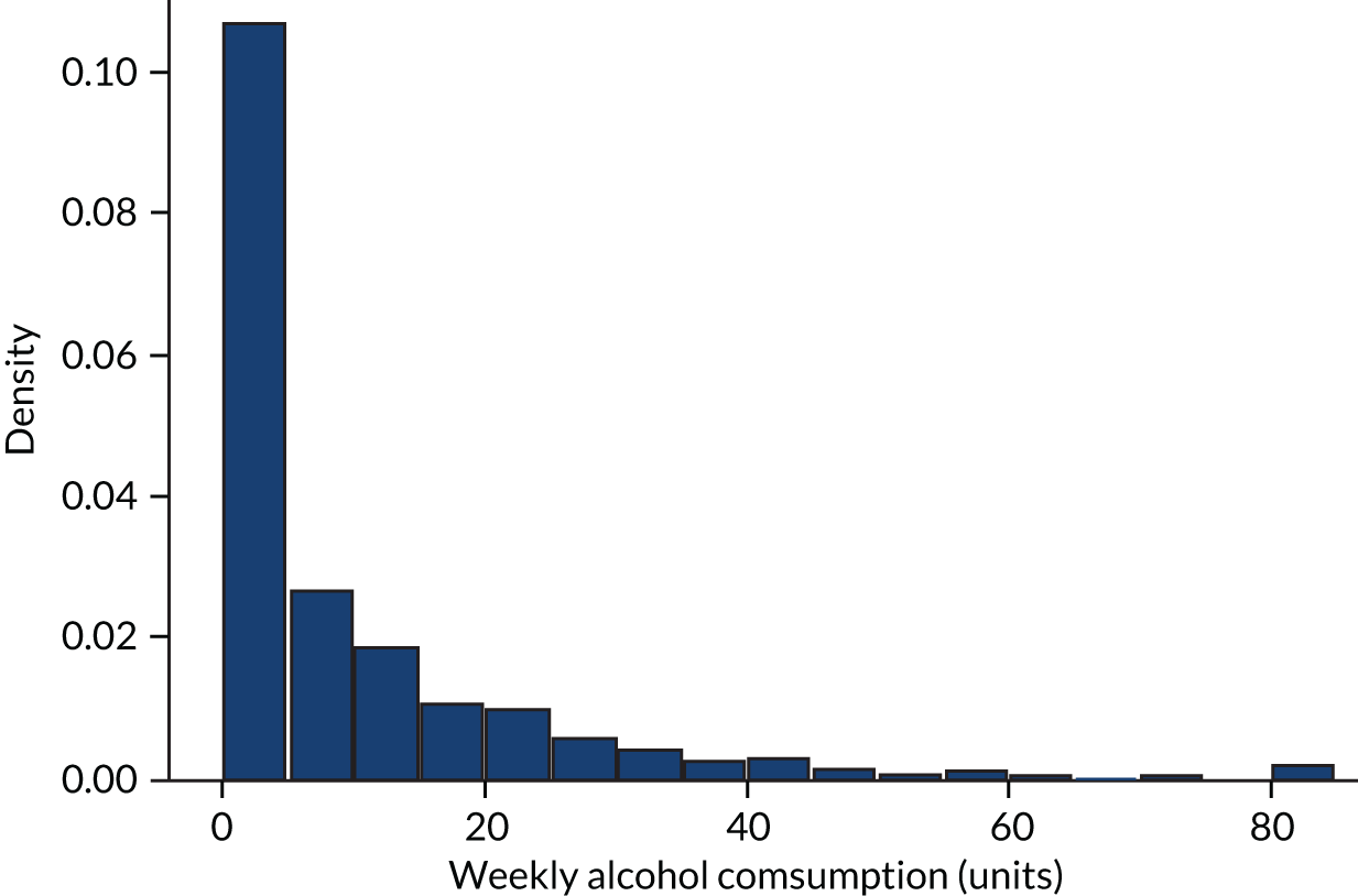
Respondents in the HSE are asked questions about their frequency of consuming, and typical consumption quantities for, several alcoholic beverages. This allows a total mean weekly alcohol consumption variable to be constructed that is measured in units of alcohol. A UK unit is 10 ml, or 8 g, of pure alcohol. The distribution of alcohol consumption in the HSE is shown in Figure 1. Seventeen per cent of the sample did not drink alcohol in the previous year, and roughly three-quarters of drinkers drank moderately (< 14 units per week). Summary statistics of the sample are presented in Table 2.
FIGURE 1.
Alcohol consumption distribution from the HSE 2011–13. Note that it is truncated at the 99th percentile.
| Characteristic | n | % |
|---|---|---|
| Total sample | 24,685 | 100.00 |
| Age band (years) | ||
| 18–24 | 1805 | 7.31 |
| 25–34 | 3706 | 15.01 |
| 35–54 | 8753 | 35.46 |
| ≥ 55 | 10,421 | 42.22 |
| Sex | ||
| Male | 10,946 | 44.34 |
| Female | 13,739 | 55.66 |
| Ethnicity | ||
| White | 22,015 | 89.18 |
| Asian | 1549 | 6.28 |
| Other | 1121 | 4.54 |
| IMD quintile | ||
| 1 (least deprived) | 5367 | 21.74 |
| 2 | 4847 | 19.64 |
| 3 | 5217 | 21.13 |
| 4 | 4770 | 19.32 |
| 5 (most deprived) | 4484 | 18.16 |
| Mean weekly alcohol consumption x (units) | ||
| 0 | 4263 | 17.27 |
| 0 < x ≤ 10 | 12,357 | 50.06 |
| 10 < x ≤ 20 | 3700 | 14.99 |
| 20 < x ≤ 30 | 2049 | 8.30 |
| 30 < x ≤ 40 | 885 | 3.59 |
| 40 < x ≤ 50 | 612 | 2.48 |
| 50 < x | 819 | 3.32 |
Each respondent’s weekly alcohol consumption was assigned to one of seven consumption bands (abstainer, or 1–10, 11–20, 21–30, 31–40, 41–50 or ≥ 51 units per week) and the probability of drinking at each consumption band was estimated using a logistic regression to predict abstention and a multinomial logistic regression to predict positive consumption bands. The multinomial logistic regression was preferred to the ordered logistic regression because it allows the most flexibility and does not impose the proportional odds assumption (for more on this, see Greene and Hensher34). These are estimated as a function of age band (18–24, 25–34, 35–54 and ≥ 55 years), sex, ethnicity (white, Asian, other), IMD quintile (the IMD is a composite measure of deprivation covering seven domains: income, employment, health, education, housing, crime and the living environment), the GOR and the alcohol-attributable hospital admissions rate and alcohol-related mortality rate for the respondent’s UTLA. 35 The admissions rates are taken from the LAPE (for more information, see www.lape.org.uk/), and are applied according to the age band and sex of the respondent. These two statistical models can be written as in Equations 1 and 2:
where iar denotes individual i in age–sex group a in UTLA r, and IMDq is the IMD quintile. Variables were treated as categorical except for HESar (the rate of alcohol-attributable hospital admission episodes per 1000 population) and MORTar (the rate of alcohol-attributable mortality per 1000 population), which were modelled as continuous variables. Using a separate logistic regression for abstention from drinking allows the direction of the coefficients to vary. For example, for a population in an area with high hospital admissions rates there may be a higher proportion likely to abstain, but also a higher proportion who drink heavily, conditional on not being an abstainer. Such divergent patterns between abstention and heavy consumption are seen in some papers in the international literature. 36 These explanatory variables are chosen because they have previously been shown to be significant predictors of alcohol consumption37 and because there are known population data for each UTLA that can be used to calculate population sizes in the subgroups defined by the combination of age, sex, ethnicity and IMD quintile. For robustness, alternative specifications of the regressions are tested, including changing the number of consumption bands (from six predefined bands to 20 equal bands, i.e. 5% in each band), and removing GOR as a predictor. These make very minor differences to the estimates in terms of mean consumption, which are shown in Appendix 1.
Once the regression parameters are estimated, these are applied for each combination of characteristics and UTLAs. For example, we calculated that the probability that a male, aged 18–24 years, of white ethnicity, in IMD quintile 3, in Sheffield, drinks 11–20 units per week is 19.6%. These probabilities are then applied to the known population data for each UTLA. The population data come from the ONS mid-year population estimates for 2013. 38 For example, there are 5196 males aged 18–24 years of white ethnicity in IMD quintile 3 in Sheffield; so we estimate that there are 1017 males aged 18–24 years of white ethnicity in IMD quintile 3 in Sheffield drinking 11–20 units per week. This calculation is performed for all combinations of characteristics and UTLAs.
These population subgroup estimates by drinker level are then used to create a new survey weight for each individual in the HSE – a survey weight specific to each UTLA. This is done by dividing the number in the UTLA population with a set of demographic characteristics and consumption band by the number of respondents with the same set of demographic characteristics and consumption band. This can be written mathematically as:
where widcr is the weight given to an individual i with demographic characteristics d and consumption band c for UTLA r; Ndcr is the number in the population with demographic characteristics d, with estimated consumption band c, in UTLA r; and ndcr is the number of HSE respondents with demographic characteristics d and consumption band c. The denominator in Equation 3 is the same for every UTLA because the number of HSE respondents by subgroup and drinker level does not differ. This now means that we can calculate 151 different weights for each individual HSE respondent – one for each UTLA. This can be used to make the HSE representative for any UTLA, and any statistic of interest on alcohol consumption can be estimated for any UTLA.
Results
Regression results
The regression results from the logistic regression for the probability of not drinking, and the multinomial logistic regression for the probability of belonging to each consumption band, are presented in Table 3. Different models were tested, including a joint model for non-drinkers and drinker bands; the methods presented here are our preferred specification. A detailed version of the methods can be found in the article by Pryce et al. 39
| Variable | Abstainer | Consumption band (mean weekly units of alcohol) | |||||
|---|---|---|---|---|---|---|---|
| 1 (0–10) | 2 (10–20) | 3 (20–30) | 4 (30–40) | 5 (40–50) | 6 (≥ 50) | ||
| Sex, age group | |||||||
| Male, 18–24 years | Reference | Reference | Reference | Reference | Reference | Reference | Reference |
| Female, 18–24 years | 0.407*** | Reference | –0.514*** | –0.533*** | –0.967*** | –0.585* | –1.017*** |
| Standard error | 0.144 | 0.143 | 0.191 | 0.260 | 0.342 | 0.278 | |
| Male, 25–34 years | –0.323** | Reference | 0.018 | 0.039 | –0.179 | –0.010 | –0.108 |
| Standard error | 0.141 | 0.122 | 0.163 | 0.203 | 0.282 | 0.207 | |
| Female, 25–34 years | 0.323** | Reference | –0.620*** | –0.772*** | –1.426*** | –0.983*** | –1.620*** |
| Standard error | 0.130 | 0.126 | 0.170 | 0.237 | 0.313 | 0.265 | |
| Male, 35–54 years | –0.064 | Reference | –0.046 | 0.359** | 0.000 | 0.382 | 0.024 |
| Standard error | 0.130 | 0.117 | 0.151 | 0.188 | 0.258 | 0.193 | |
| Female, 35–54 years | 0.318*** | Reference | –0.511*** | –0.570*** | –1.018*** | –0.656** | –1.042*** |
| Standard error | 0.119 | 0.110 | 0.147 | 0.185 | 0.258 | 0.193 | |
| Male, ≥ 55 years | 0.390** | Reference | –0.274* | 0.250 | –0.128 | 0.211 | –0.232 |
| Standard error | 0.157 | 0.145 | 0.184 | 0.241 | 0.308 | 0.239 | |
| Female, ≥ 55 years | 1.163*** | Reference | –0.791*** | –0.736*** | –1.399*** | –0.744*** | –1.846*** |
| Standard error | 0.117 | 0.110 | 0.146 | 0.189 | 0.256 | 0.213 | |
| IMD quintile | |||||||
| 1 (least deprived) | Reference | Reference | Reference | Reference | Reference | Reference | Reference |
| 2 | 0.186*** | Reference | –0.057 | 0.047 | –0.056 | –0.013 | –0.113 |
| Standard error | 0.065 | 0.057 | 0.071 | 0.102 | 0.128 | 0.114 | |
| 3 | 0.334*** | Reference | –0.106* | –0.158** | –0.234** | 0.015 | –0.121 |
| Standard error | 0.062 | 0.056 | 0.074 | 0.106 | 0.126 | 0.113 | |
| 4 | 0.615*** | Reference | –0.226*** | –0.144* | –0.311*** | –0.064 | –0.137 |
| Standard error | 0.062 | 0.061 | 0.078 | 0.113 | 0.136 | 0.118 | |
| 5 (most deprived) | 1.003*** | Reference | –0.384*** | –0.188** | –0.409*** | 0.032 | –0.052 |
| Standard error | 0.063 | 0.068 | 0.086 | 0.126 | 0.144 | 0.123 | |
| GOR | |||||||
| North East | Reference | Reference | Reference | Reference | Reference | Reference | Reference |
| North West | 0.056 | Reference | –0.053 | –0.136 | –0.416*** | 0.032 | –0.381*** |
| Standard error | 0.078 | 0.084 | 0.105 | 0.146 | 0.178 | 0.138 | |
| Yorkshire and the Humber | 0.152* | Reference | –0.155 | –0.253** | –0.473*** | –0.074 | –0.562*** |
| Standard error | 0.086 | 0.096 | 0.119 | 0.168 | 0.199 | 0.167 | |
| East Midlands | –0.182* | Reference | –0.024 | –0.404*** | –0.472*** | –0.271 | –0.464*** |
| Standard error | 0.095 | 0.097 | 0.127 | 0.173 | 0.214 | 0.172 | |
| West Midlands | –0.068 | Reference | –0.077 | –0.258** | –0.384** | –0.212 | –0.321** |
| Standard error | 0.087 | 0.093 | 0.117 | 0.161 | 0.202 | 0.156 | |
| East of England | –0.128 | Reference | –0.303*** | –0.525*** | –0.821*** | –0.605*** | –0.754*** |
| Standard error | 0.101 | 0.106 | 0.133 | 0.192 | 0.233 | 0.191 | |
| London | –0.201 | Reference | 0.021 | –0.451*** | –0.527** | –0.805*** | –0.847*** |
| Standard error | 0.124 | 0.135 | 0.173 | 0.247 | 0.299 | 0.256 | |
| South East | –0.116 | Reference | –0.056 | –0.214* | –0.545*** | –0.278 | –0.539*** |
| Standard error | 0.093 | 0.097 | 0.122 | 0.173 | 0.212 | 0.172 | |
| South West | –0.087 | Reference | –0.108 | –0.287** | –0.507*** | –0.426** | –0.787*** |
| Standard error | 0.093 | 0.094 | 0.118 | 0.165 | 0.212 | 0.176 | |
| Ethnicity | |||||||
| White | Reference | Reference | Reference | Reference | Reference | Reference | Reference |
| Asian | 2.600*** | Reference | –0.887*** | –1.098*** | –1.328*** | –1.082*** | –1.542*** |
| Standard error | 0.063 | 0.134 | 0.193 | 0.311 | 0.343 | 0.362 | |
| Other | 1.436*** | Reference | –0.757*** | –0.936*** | –0.722*** | –0.992*** | –0.644*** |
| Standard error | 0.072 | 0.126 | 0.178 | 0.242 | 0.328 | 0.249 | |
| Local characteristics | |||||||
| Alcohol-attributable hospital admissions | 11.107 | Reference | 32.382 | –0.832 | 0.656 | 49.493 | 64.317* |
| Standard error | 20.358 | 20.374 | 25.058 | 35.363 | 39.557 | 33.360 | |
| Alcohol-related mortality | –501.222 | Reference | –80.800 | –1344.139** | –876.633 | –2981.573*** | –379.819 |
| Standard error | 429.614 | 465.335 | 595.386 | 875.668 | 1016.384 | 860.621 | |
| Constant | –2.622*** | Reference | –0.672*** | –0.589* | –0.932** | –1.433** | –1.610*** |
| Standard error | 0.255 | 0.258 | 0.333 | 0.472 | 0.572 | 0.466 | |
| Observations (n) | 24,685 | 20,422 | 20,422 | 20,422 | 20,422 | 20,422 | 20,422 |
The results from the logistic regression show that abstention rates are higher in females across all age ranges (a positive coefficient indicates greater likelihood of being an abstainer than for the reference category), and that older males are more likely to abstain than younger males. Those in the most deprived quintile are most likely to abstain, and the relationship between deprivation quintile and abstention probability is monotonic. There is slight variation across GORs, but the main predictor of abstention is ethnicity, with those of Asian ethnicity most likely to abstain. Those of white ethnicity are least likely to abstain. Neither alcohol-attributable hospital admissions nor mortality are significant predictors of abstention.
The results from the multinomial logistic regression for consumption band show that females are less likely to be in the highest consumption bands than males, but, unlike abstention, there is no significant difference between older and younger males. The least deprived (people in more affluent areas) are more likely to be in higher consumption bands than those from poorer areas. Unlike abstention, there is large regional variation in consumption bands, with the North East reference category most likely to be in higher consumption bands, followed by the North West. Again, ethnicity is a significant predictor of alcohol consumption, with those of Asian ethnicity much less likely to be in a higher consumption band, even among those who drink alcohol. The local authority-level alcohol-attributable hospital admissions rate variable is significantly related to greater probability of being in the highest consumption band and the trend looks somewhat ‘U-shaped’, that is in areas with higher admissions there is a greater chance of being in the lower consumption or higher consumption bands, and less chance of being in the mid-range consumption bands (although some of these coefficients are not significantly different from zero). In contrast, mortality is negatively and significantly related to the probability of being in the highest consumption band, which may be counterbalancing the coefficient on hospital admissions, as these variables are correlated.
Local authority variation
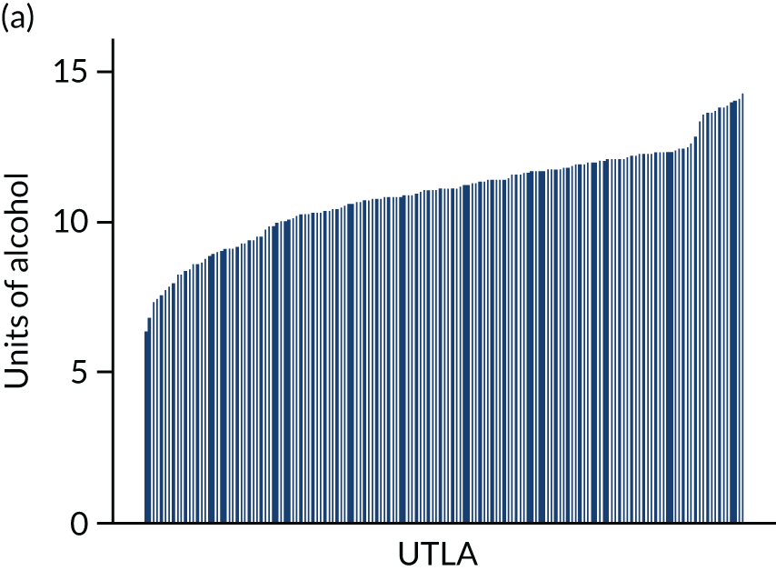
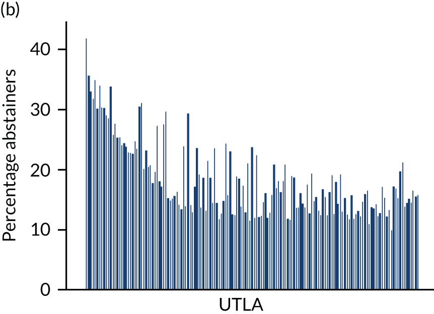
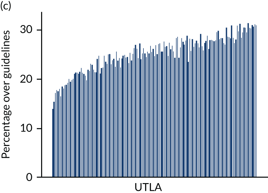
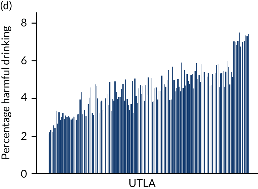
Four consumption metrics for each UTLA are shown in Figure 2. There is variation in the estimates of mean weekly consumption across UTLAs, with twofold variation between the lowest estimates (around 7 units per week) and the highest (around 14 units per week). Abstention estimates again show large variation across UTLAs, from as low as 11% to as high as 42%, which is probably driven by variation in ethnicity. Because the x-axis is sorted by mean consumption estimate, it shows that there is correlation between abstention and mean consumption, but that some areas have high abstention and high mean consumption. The estimates for the proportion of people drinking more than the recent Chief Medical Officers’ guidelines40,41 of 14 units vary from around 13% of the population to > 30%. Estimates for those drinking at a harmful rate (high-risk drinking is classified as drinking > 35 units per week for females and > 50 units per week for males) vary from around 2% to almost 8% of the population, and both high-risk drinking and increasing-risk drinking (over the Chief Medical Officer’s guidelines) are strongly correlated with the mean consumption estimates.
FIGURE 2.
Estimated consumption metrics based on method to produce synthetic re-weighted survey for each UTLA in England, sorted by mean consumption. (a) Mean consumption; (b) abstention; (c) more than the guidelines recommend; and (d) harmful drinking.
Comparison with observed data
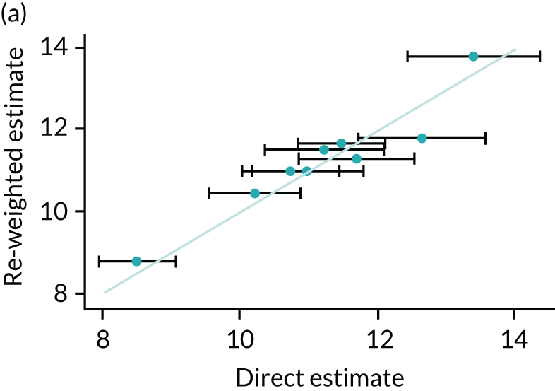
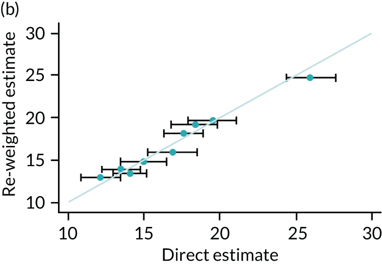
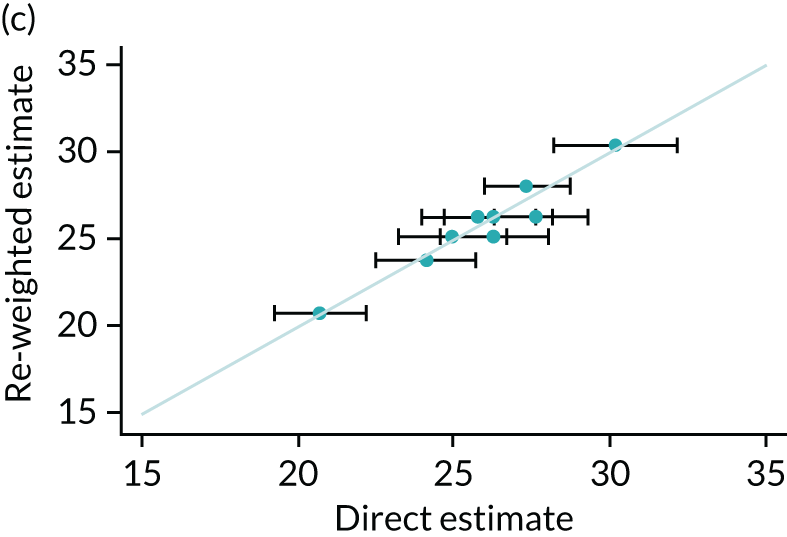
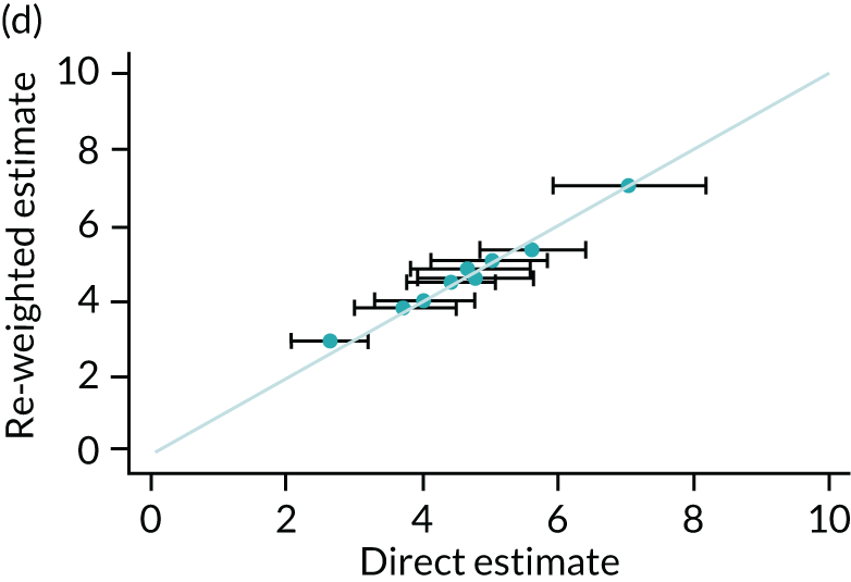
One method of validation is to compare results generated from the re-weighting method with directly measured statistics at GOR level, as the HSE is designed to be representative at this level. Four scatterplots comparing re-weighted estimates with direct measures are presented in Figure 3. The model performs very well at predicting GOR-level estimates, with all estimates lying within the 95% confidence intervals calculated from the observed data. The correlation coefficient between re-weighted estimates and GOR-level direct measures are 0.95, 0.98, 0.82, and 0.99 for mean consumption, abstention, more than the guidelines recommend and harmful drinking, respectively.
FIGURE 3.
Comparison between re-weighted estimates and HSE data at region level. (a) Mean consumption; (b) abstention; (c) more than the guidelines recommend; and (d) harmful drinking.
Discussion
This section has presented a method of re-weighting nationally representative data so that they are representative at the local authority level, in this case constructing 151 locally representative versions of the HSE. This was done by estimating the population of each local authority according to age band, sex, ethnicity, IMD and alcohol consumption. Dividing the number of people with these characteristics in each local authority population by the number of respondents with the same characteristics in the survey gives a new survey weight. To our knowledge, this is the first paper to re-weight the HSE data to obtain local survey data on alcohol use, and, to our knowledge, the first to use such an approach to develop local estimates of alcohol consumption distributions anywhere in the world. The findings show substantial variation in estimated alcohol consumption and abstention rates across UTLAs with a 4.5-fold variation in the estimated abstention rates and a twofold variation in the estimated mean consumption. The results are stable across the alternative specifications of statistical models, as shown in Appendix 1.
Local authorities need to be aware of the variation in estimated drinking volumes, given that there are several policy options, such as licensing decisions and provision of screening and brief interventions, which are decided at the local level. Despite the limitations of the models, the results have clear potential to be used by local decision-makers. The model fit, compared with direct estimates at the GOR level, is excellent. A potentially useful feature of the re-weighting method is that an estimate of the dependent variable (i.e. consumption) can be obtained for any cut-off point – so that policy-makers could estimate how many people drink more than any number of units in their area. Individual areas may also wish to use these estimates for benchmarking and perhaps plan or prioritise services accordingly. The re-weighted HSE data can be used, in conjunction with other local data sources, to model local policy interventions. Given the heterogeneous effects of policies across population subgroups, the capability of the new methods to enable local-level modelling of outcomes for subgroups stratified by age, sex and social deprivation is especially important.
There are several limitations to the method presented, as well as some assumptions that will carry through to any modelling work. Perhaps the most important assumption is that the statistical relationship between the left- and right-hand side variables is constant across the UTLAs; the effect on consumption of being male, for example, is assumed to be similar across all UTLAs. However, this is always implicitly the case with survey weights more generally, in that survey respondents are representative of their sample frame. Furthermore, caution is required when looking at variables not included in the analysis, such as, in this case, smoking habits. These wider attributes of the respondents have not been modelled here, and may differ by UTLA. In addition, the statistical re-weighting analysis method presented here examines the level of mean weekly consumption and does not disentangle drinking patterns and beverage type when undertaking the re-weighting. That is not to say that analysis of this type is not feasible, simply that further work could address this issue through the inclusion of exogenous local data on beverage preferences. Further work could also look at why people in some regions of England drink more than people in other regions, even when controlling for explanatory factors including demographics and hospitalisation rates. This has been noted in the existing literature. 37
There are several implications for future related research. First, more detailed validation against external data would require locally representative data to be collected. This is not easy. Public Health England has conducted surveys in 25 UTLAs to get a measure of local consumption. 42 The re-weighted method correlates moderately well, but the sample size of the local surveys is not large enough to be sufficient. Extensions of this work could provide updates when new data become available, or look at other health risk factors such as smoking or obesity. Combinations of behaviours, to allow multibehaviour modelling, could be analysed. Harm risks are particularly acute when individuals have multiple unhealthy behaviours, as the risks are multiplicative, and unhealthy behaviours tend to cluster within individuals. 43 Furthermore, the method of re-weighting presented in this paper is not unique to either alcohol or small geographical areas, and can be applied to a whole host of outcomes, estimates of which are not directly available for small populations. None of this analysis has looked at geography in the UTLA boundary, for example at electoral ward level or even finer geographies that could relate to specific licensing decisions for on-trade or off-trade outlets.
In conclusion, this section finds that re-weighting nationally representative surveys to make them representative at the local level is possible and also finds large variation in alcohol abstention, mean consumption and measures of heavy drinking across UTLAs. The results of the estimation when aggregated up to provide GOR estimates align closely with directly observed data. This method could be used in any country where national survey data are available and could be applied to many other outcomes of public health interest to inform local priorities and decisions.
Estimating beverage preferences and the distribution of prices paid for each local authority by beverage category and population subgroup
Introduction
A fundamental requirement for modelling the local effect of minimum unit pricing is estimates of the price distribution at the local level. This is because there is good reason to suspect that prices paid for alcoholic beverages differ across localities, partly for demand-side reasons (differing population characteristics, different drink preferences) and partly for supply-side reasons (differing rental prices, differing levels of competition among suppliers).
Preferences are also likely to vary across the country because of differing population characteristics and some underlying regional cultural preferences; for example, cider is typically consumed at higher levels in the South West. Preferences are important for modelling the local effect of minimum unit pricing because different drinks will be affected at different levels. Perhaps most important is the split between on-premise (pubs, bars and restaurants) and off-premise (shops and supermarkets), because the on-premise market is barely affected by minimum unit pricing.
For local alcohol price estimates, we estimated the prices currently paid for 10 beverage categories: beer, cider, wine, spirits and RTDs, split by off-trade (supermarkets and shops) and on-trade (pubs, bars etc.). This required synthesis of evidence from the LCFS and market research data. The market research data were provided by CGA (CGA Strategy Ltd, Stockport, UK) and Nielsen (Nielsen Holdings plc, New York, NY, USA) at GOR level. We needed these data because it is known that the amount of alcohol bought in each price band as reported by respondents to the LCFS is slightly different from the evidence available from retail sales data. Typically, the LCFS underestimates the amount of cheap alcohol being sold, and so the methods developed and applied here allow us to adjust for this underestimation for each UTLA.
In terms of subgroups, for both price distributions and preferences, we estimate results for 120 different population subgroups. These are based on two sexes, four age groups (18–24, 25–34, 35–54 and ≥ 55 years), five quintiles of IMD and three groups based on the amount of alcohol purchased in the 2-week diary window (moderate, increasing risk and high risk).
Data sources: the Living Costs and Food Survey calibrated to market research company sales data
The price distributions are estimated using the LCFS 2012–14, accessed via the UK Data Service Secure Lab. The LCFS is a nationally representative survey that requires respondents to complete a 2-week purchasing diary of all items, including alcohol. We analysed 10,065 individuals with 57,581 alcohol transactions in the years 2012–14 in England. The data are available at transaction level, meaning that we see the price paid for every item. The LCFS also records the demographic characteristics of the respondent, including their age and sex, IMD quintile and income quintile. The secure version of the data allows us to see the UTLA of residence, which means characteristics of the local area can be merged in as explanatory variables in the statistical model.
Data on UTLA area characteristics were merged with the UK Data Service Secure Lab transaction records from three sources. The first was data on hospital admission rates by UTLA, taken from the LAPE. 4 The second source was data on outlet density rates, provided by the market research company CGA for each UTLA. The outlet density is defined as the mean number of outlets selling alcohol within 1 km of a postcode in the UTLA, based on data from 2013. 24 The third source was data on the average house prices in the UTLA, which are taken from the Land Registry. 44
The estimated price distributions are calibrated using market research data from CGA (on-premise) and Nielsen (off-premise). The market research data do not provide any information on who is buying alcohol at certain price points; instead, they provide information on the total volume of sales at different price bands (i.e. the price distribution of alcohol prices in each GOR for each of the 10 beverage categories). The data were provided at TV region level, which broadly maps on to GOR. The off-trade data from Nielsen provide price distributions, in bands of 5p, up to £1.20 per unit of alcohol, whereas the on-trade data from CGA are in 5p bands up to £1.20 per unit of alcohol and in 10p bands from £1.20 to £2.60 per unit of alcohol. Both sets of data include an open category for sales above the highest price band and relate to alcohol sold in 2016.
The preferences for different categories of alcohol for each UTLA and population subgroup are estimated using just the LCFS data set. This is because, unlike price distributions, there was no local authority variable that could easily be justified to predict preferences. This is compounded by the fact that preferences are non-ordinal, meaning that patterns in the data cannot be used as easily. The preference vectors are taken empirically from the LCFS 2010–15. This provided more observations – a total of 25,186 individuals with 116,408 alcohol transactions – although it did not include information on the UTLA of residence. The data are, again, available at transaction level, meaning that we can get information on the amount, in ml, purchased. These volumes are converted to units of alcohol using standard assumptions about alcoholic strength, which are set out in Appendix 2.
Method for estimating preferences for the 10 beverage categories
The method employed to estimate preference vectors for each subgroup can be broken down into three stages. The preference vectors are taken empirically from the data.
The aim was to get a preference vector (the proportion of purchased alcohol that is in each of the 10 beverage categories) for each of 120 population subgroups in each UTLA. For example, for males aged 35–54 years, in IMD quintile 3, drinking at high-risk levels, in the Sefton UTLA. If we wanted to calculate the proportion of alcohol purchased in each of the 10 categories, we might find that it was as follows: off-trade beer, 25%; off-trade cider, 5%; off-trade wine, 10%; off-trade spirits, 20%; off-trade RTDs, 1%; on-trade beer, 20%; on-trade cider, 3%; on-trade wine, 5%; on-trade spirits, 10%; and on-trade RTDs, 1%, which adds up to 100%.
To do this, we followed these steps:
-
Transaction-level LCFS data from 2010–15 were cleaned and processed. Purchases were split into the 10 beverage categories (beer, cider, wine, spirits, RTDs, both on- and off-premise). We use this to calculate a preference vector (the 10 percentages) for the whole adult population of England.
-
Next, we divided the sample population into subgroups to get preferences for each subgroup. This was done in stages. The sample was first divided by the nine GORs, as this was chosen as the most important driver of preferences. Thus, we have nine preference vectors, one for each GOR for all adults. The sample is then divided by three drinker types (moderate, increasing risk, high risk), as different drinker types are likely to have different preferences. For example, heavier drinkers tend to drink proportionally more cider and spirits, and less on-premise alcohol. Therefore, we now have 9 × 3 preference vectors. The sample is then divided by sex, as men and women are likely to drink different beverages; for example, women drink a higher proportion of wine. We now have the proportion of alcohol purchased split into the 10 beverage categories for 54 subgroups (nine regions, by three drinker types, by two sexes). The data are disaggregated further only if subgroups have ≥ 50 transactions, as fewer than this would not give a robust preference split. Some subgroups are able to be disaggregated by age band to give region–drinker–sex–age preference vectors.
-
Finally, the preference vectors are applied to the re-weighted consumption estimates (using a method detailed in Method to combine the preference and price distribution modelling with the re-weighted consumption estimates) to give local UTLA consumption estimates broken down into the 10 beverage categories.
Methods for statistical modelling to estimate price distributions
The method employed to estimate price distributions for each subgroup in each UTLA for each beverage type can be broken down into the following stages.
Ordinal logistic regression models for the probability that a transaction falls within each of 50 price bands, defined by price per unit of alcohol
First, transaction-level LCFS data from 2012–14, which contain rich purchasing information by individuals, were cleaned and processed. The price per unit of alcohol was calculated using assumptions around the strengths of products purchased. These assumptions can be found in Appendix 2.
Second, a statistical model was built that estimates the probability of the transaction price falling into one of 50 price-per-unit bands. The price bands are equal-width, 5p bands; the lowest band is ‘< £0.05 per unit’ and the top band is ‘≥ £2.45 per unit’. The statistical model uses individual-level characteristics [i.e. age band (18–24, 25–34, 35–54 and ≥ 55 years), sex, income quintile and drinker type (moderate, increasing risk, high risk)] and local area-level variables (i.e. outlet density at UTLA level; alcohol-attributable hospital admissions at UTLA level, split by age band and sex; and average house prices at GOR level).
The statistical model used to estimate the price distributions is an ordered logistic regression. This accounts for the ordinal nature of the price bands. Sex and age band are combined to give eight explanatory sex–age groups. A statistical model for each beverage type is estimated separately, so that there are 10 statistical models.
Alternative model specifications
We tested other mathematical forms for the statistical modelling, including multinomial regression. The results are not shown here. The ordinal regression method had better statistical fit.
Method to combine the preference and price distribution modelling with the re-weighted consumption estimates
Once the statistical models were estimated, the resulting proportions were applied to the re-weighted consumption data with beverage splits, to give local consumption estimates broken down into 10 beverage categories and 50 price bands.
This was done by selecting a subgroup to analyse, and then adding the total re-weighted consumption (calculated as shown in Local authority variation) of all the individuals in that subgroup in the UTLA. We then applied the proportions in each of the 10 beverage categories (see Method for estimating preferences for the 10 beverage categories) to that total consumption, giving the number of units consumed in 1 year in each beverage category by that subgroup in that UTLA. Next, we applied the price distribution estimate for the subgroup for each beverage category (see Ordinal logistic regression models for the probability that a transaction falls within each of 50 price bands, defined by price per unit of alcohol), so that we had the estimated number of units of each beverage category of alcohol consumed that were purchased in each of the 50 price bands. This gave us, for example, an estimate of how many units of off-trade beer were consumed by males aged 35–54 years, in IMD quintile 3, who are moderate drinkers, that were purchased at a price of between 40p and 45p per unit of alcohol in the Sefton UTLA.
This process was repeated for each subgroup.
We then generated a total for the UTLA population, showing the number of units of each of the 10 beverage categories consumed, split by the 50 price bands, for example to estimate how many units of off-trade beer were consumed that were purchased at a price of between 40p and 45p per unit of alcohol in the Sefton UTLA.
Method to calibrate to market research company price distributions
Finally, the price distributions for each beverage category in each of the UTLAs in the North West region were aggregated up to GOR level and compared with the market research data supplied by CGA and Nielsen. This comparison was used to calibrate, at the beverage level, to the market research data.
The process involved redefining the 50 price band boundaries such that the LCFS price distributions matched the market research data. This has the principal advantage that it corrects the price distribution to observed levels without distorting the relative price distributions across individual-level characteristics.
Consider the following example: imagine that we have estimated that 5.0% of all off-premise beer purchases in the North West fall into the LCFS price band 11, corresponding to 50–55p per unit of alcohol. Moreover, imagine that we have also estimated that 40.0% of all the off-premise beer in the North West is sold at < 50p per unit of alcohol; thus, 45.0% of all off-premise beer is sold at < 55p per unit. To calibrate this, we take the price point corresponding to the 40th percentile of Nielsen’s price distribution for the North West (imagine that this is actually 47.5p), and the price point corresponding to the 45th percentile (imagine that this is 53p per unit). These are the price points to which the data are calibrated. What this means, in practice, is that every transaction that, in the LCFS, falls into price band 11 is actually priced at between 47.5p and 53p.
Results of price distributions analyses
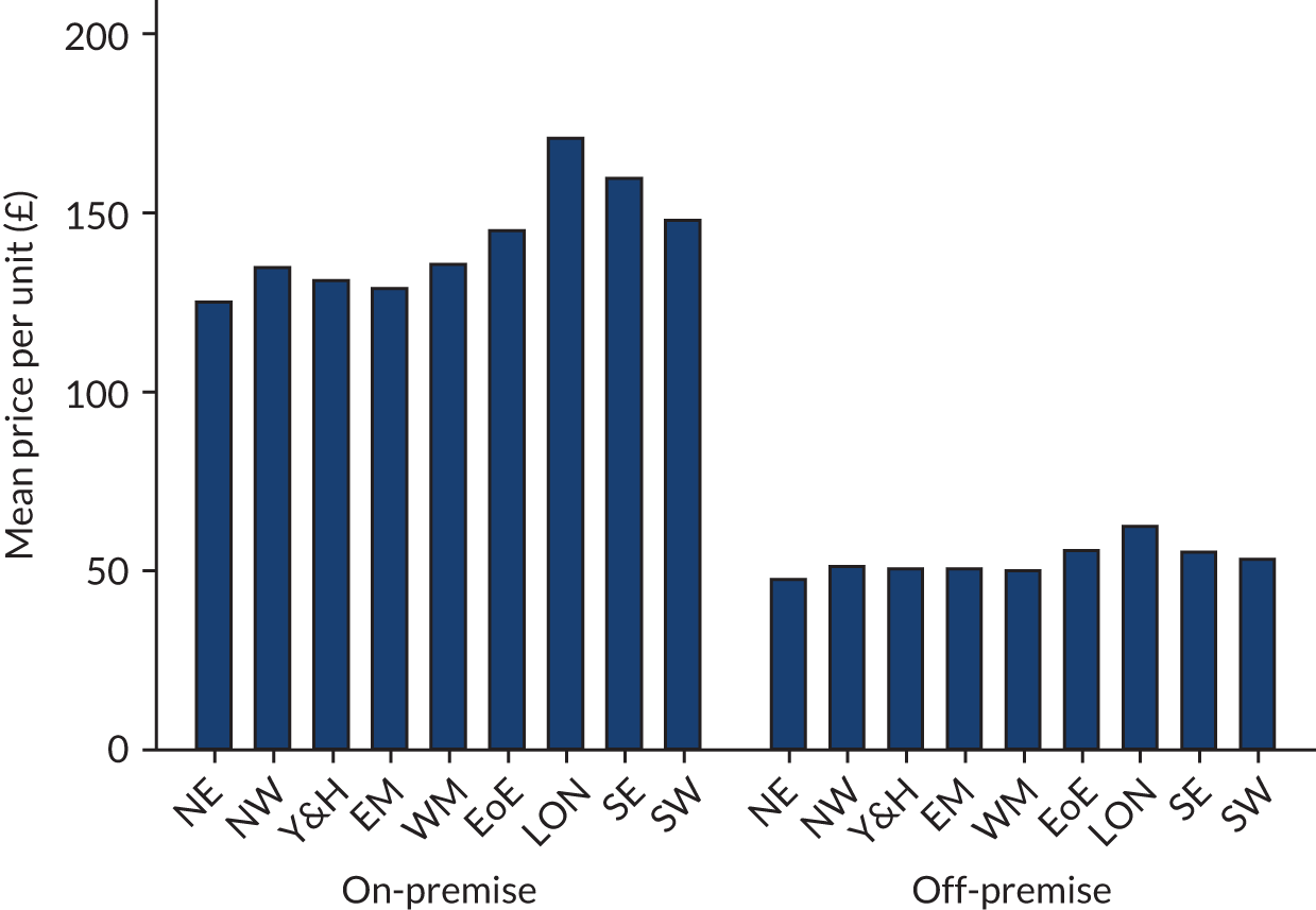
Figure 4 shows the mean price per unit of alcohol in each region, split by on-trade and off-trade, from the raw LCFS secure data. It shows that there is a large difference in prices between on-premise and off-premise beverages. It also shows that there is more across-GOR variation in on-premise prices than in off-premise prices. The most expensive mean price per unit is in London for both on-premise and off-premise, whereas the cheapest mean price per unit is in the North East for both on-premise and off-premise. The variation in the mean price per unit arises from both preference (e.g. Londoners may drink more champagne, which is expensive) and price differences (e.g. Londoners purchase more expensive wine when they purchase wine).
FIGURE 4.
The mean price per unit in each region, split by on-trade and off-trade, from raw LCFS data. EM, East Midlands; EoE, East of England; LON, London; NE, North East; NW, North West; SE, South East; SW, South West; Y&H, Yorkshire and the Humber; WM, West Midlands.
The regression results are presented in Appendix 3, Tables 12 and 13, for on-premise and off-premise, respectively. The results are regression parameters, so their magnitude cannot be directly assessed from the table, but the direction can.
For on-premise alcohol, the results in Appendix 3, Table 12, show that the youngest age group tend to pay less per unit than their elder counterparts. Similarly, and perhaps as expected, price paid per unit increases as income increases. High-risk drinkers tend to spend significantly less per unit on on-premise alcohol. The outlet density in the UTLA has a mixed effect on price paid. In contrast, higher hospital admission rates tend to reduce the amount paid per unit of on-premise alcohol. Higher average house prices increase the price paid per unit of on-premise alcohol, reflecting higher on-premise property costs being passed on to consumers.
For off-premise alcohol, sales of which are affected more by a MUP than on-premise alcohol sales, Appendix 3, Table 13, shows a similar pattern in terms of age and income: younger people and those who are less well-off tend to pay lower prices. Most importantly, high-risk and increasing-risk drinkers spend significantly less per unit on alcohol, after controlling for beverage choice. The outlet density tends to be an insignificant explanatory variable in the off-premise category, except for off-premise cider. Hospital admission rates and average house prices are significant predictors of the price paid for off-premise alcohol, with people in areas with higher hospital admission rates and lower house prices tending to pay less for their shop-bought alcohol.
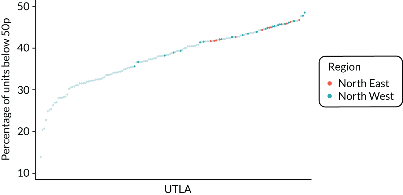
Figure 5 shows the variation in the percentage of units purchased at < 50p in the uncalibrated estimates. It shows that there is substantial variation across UTLAs, and that the North East and North West of England have some of the highest proportions of alcohol purchased that comes under the potential 50p MUP. Although the price distribution estimates match the raw LCFS data fairly well at GOR level, there is concern that the LCFS data may routinely under- or over-report purchases of cheap alcohol as a result of measurement error.
FIGURE 5.
Uncalibrated price distribution estimates.
Figures 6 and 7 show kernel density graphs of the cumulative price distributions from the statistical model and the market research data at the GOR level for the North West and North East, respectively. The estimates from the statistical model are then calibrated so that the cumulative distributions match.
FIGURE 6.
Comparison of price estimates with market research data: North West. (a) On-premise beer; (b) on-premise cider; (c) on-premise wine; (d) on-premise sprits; (e) on-premise RTDs; (f) off-premise beer; (g) off-premise cider; (h) off-premise wine; (i) off-premise sprits; and (j) off-premise RTDs.
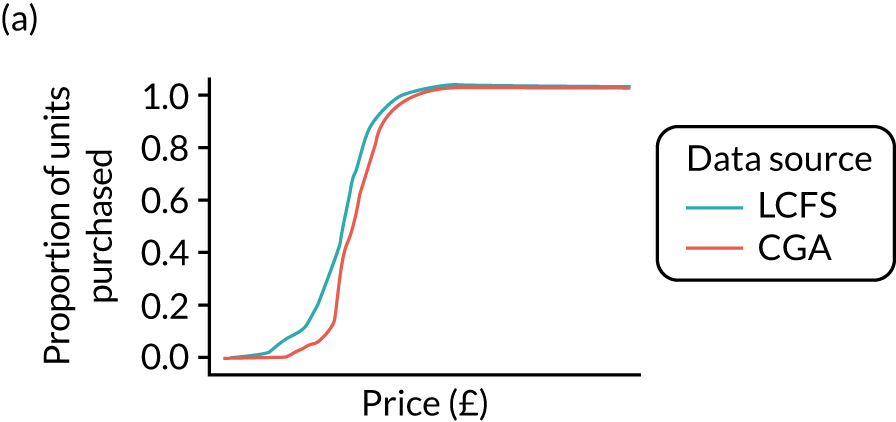
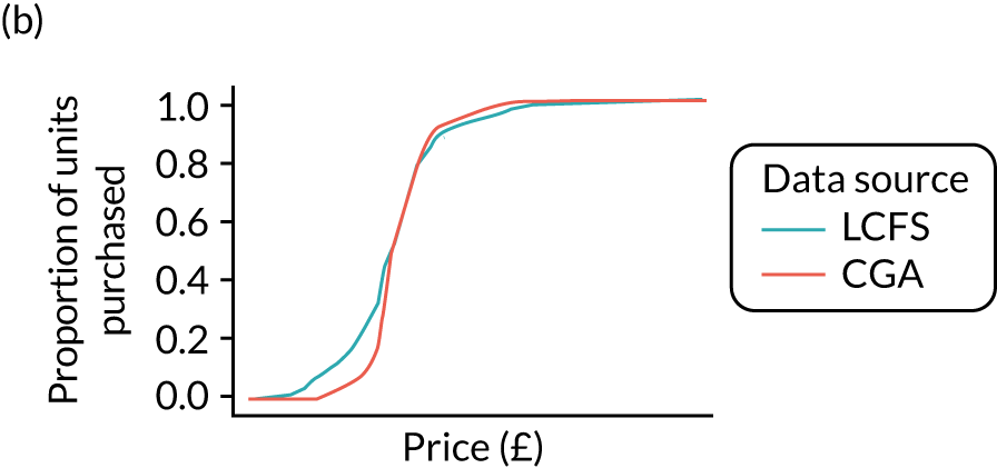
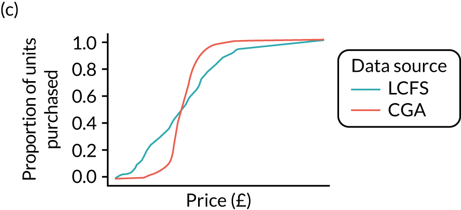
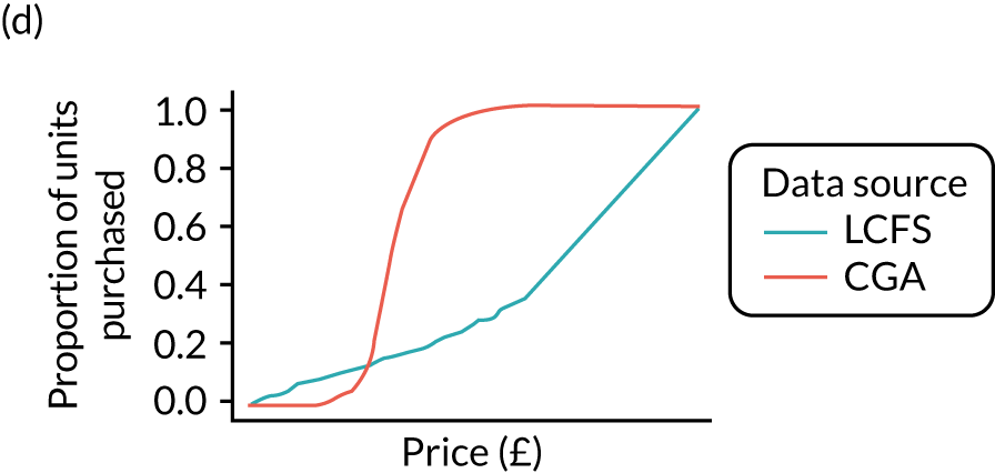
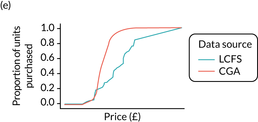
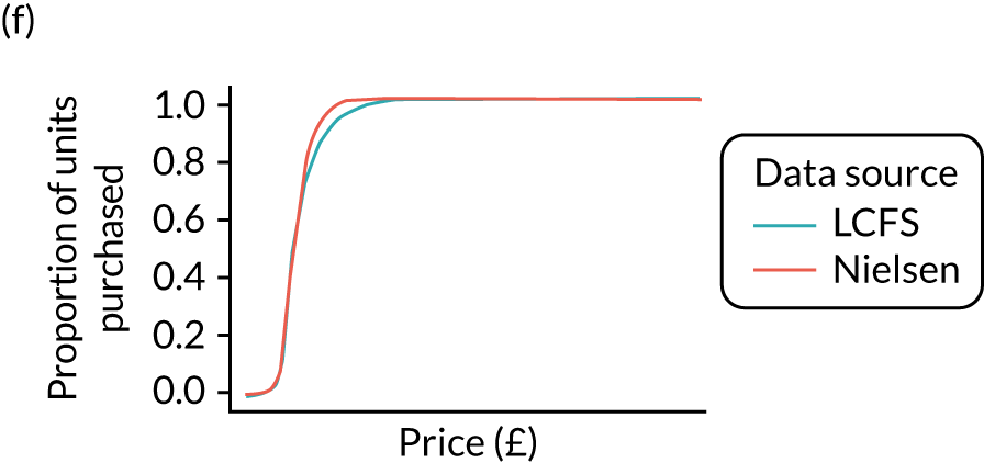
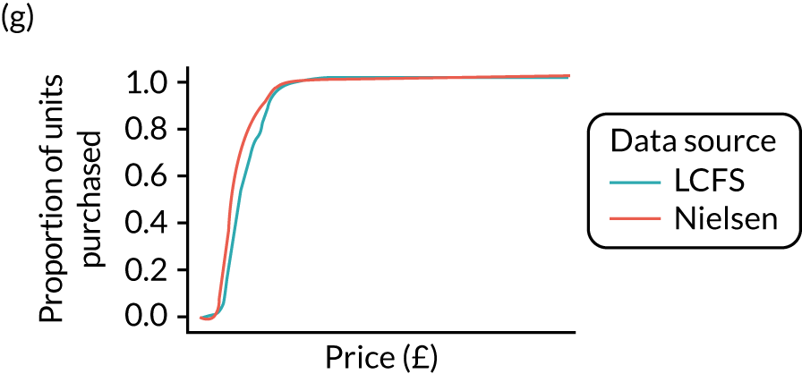
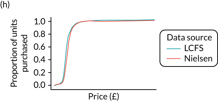
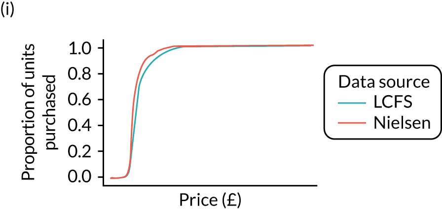
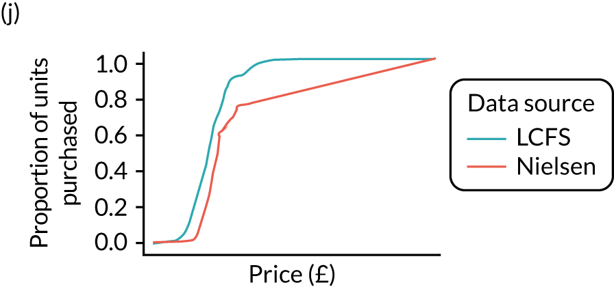
FIGURE 7.
Comparison of price estimates with market research data: North East. (a) On-premise beer; (b) on-premise cider; (c) on-premise wine; (d) on-premise sprits; (e) on-premise RTDs; (f) off-premise beer; (g) off-premise cider; (h) off-premise wine; (i) off-premise sprits; and (j) off-premise RTDs.
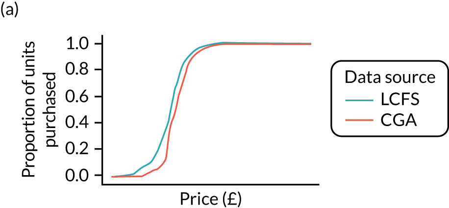
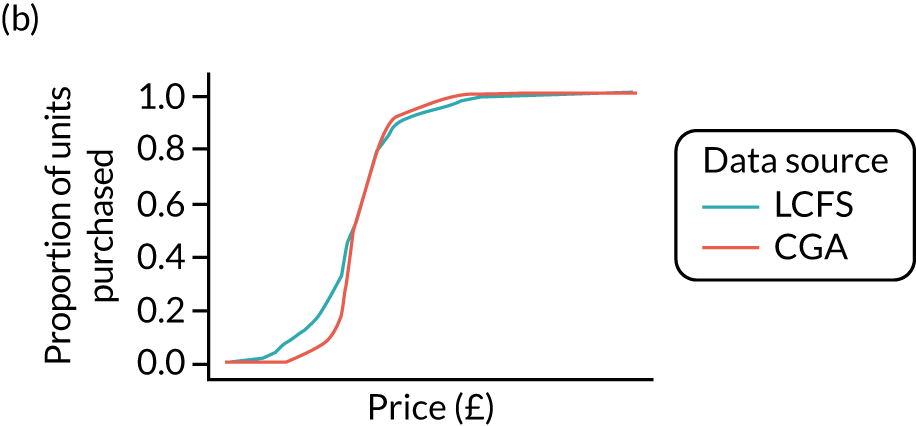
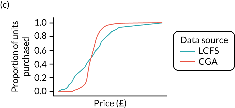
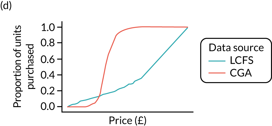
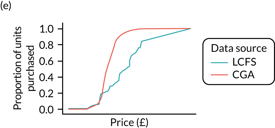
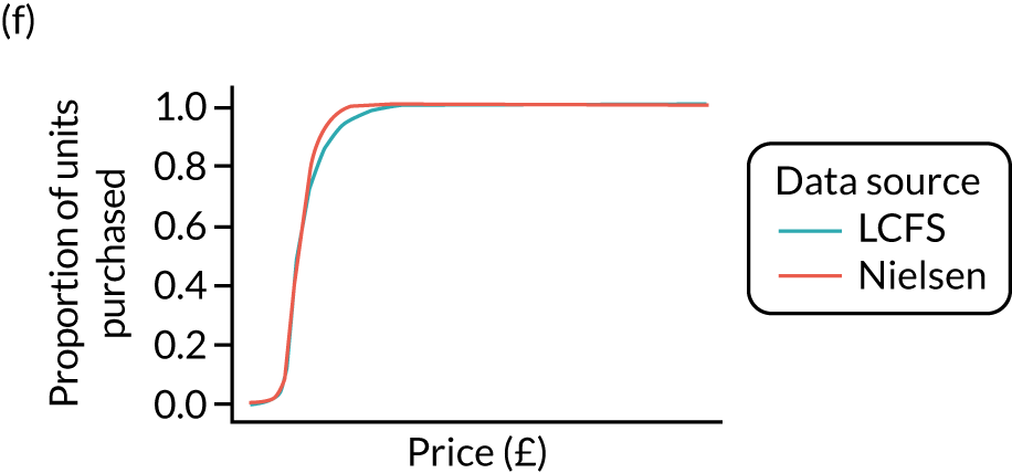
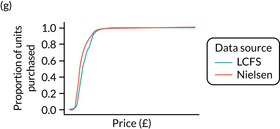
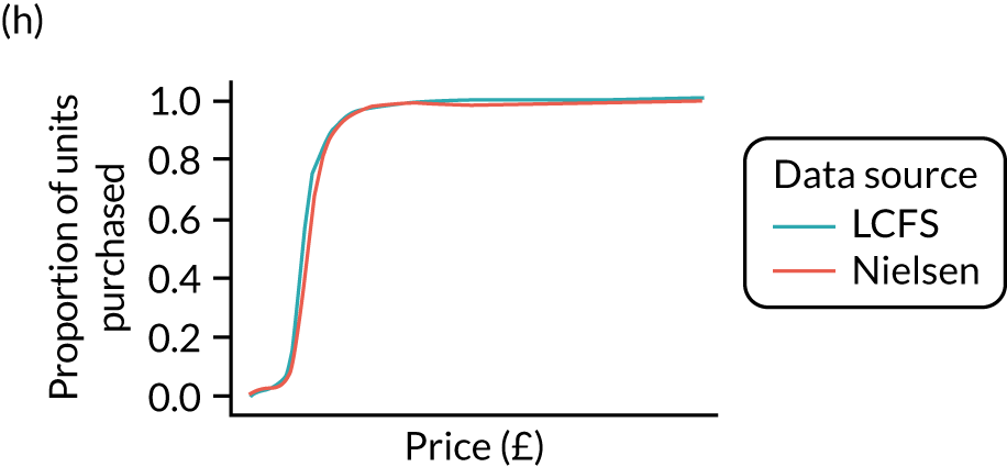
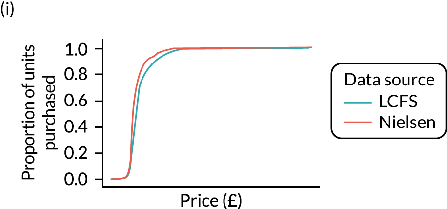
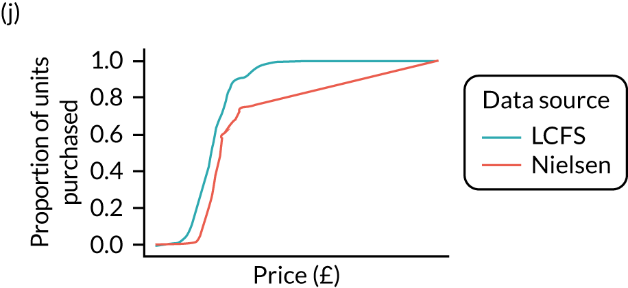
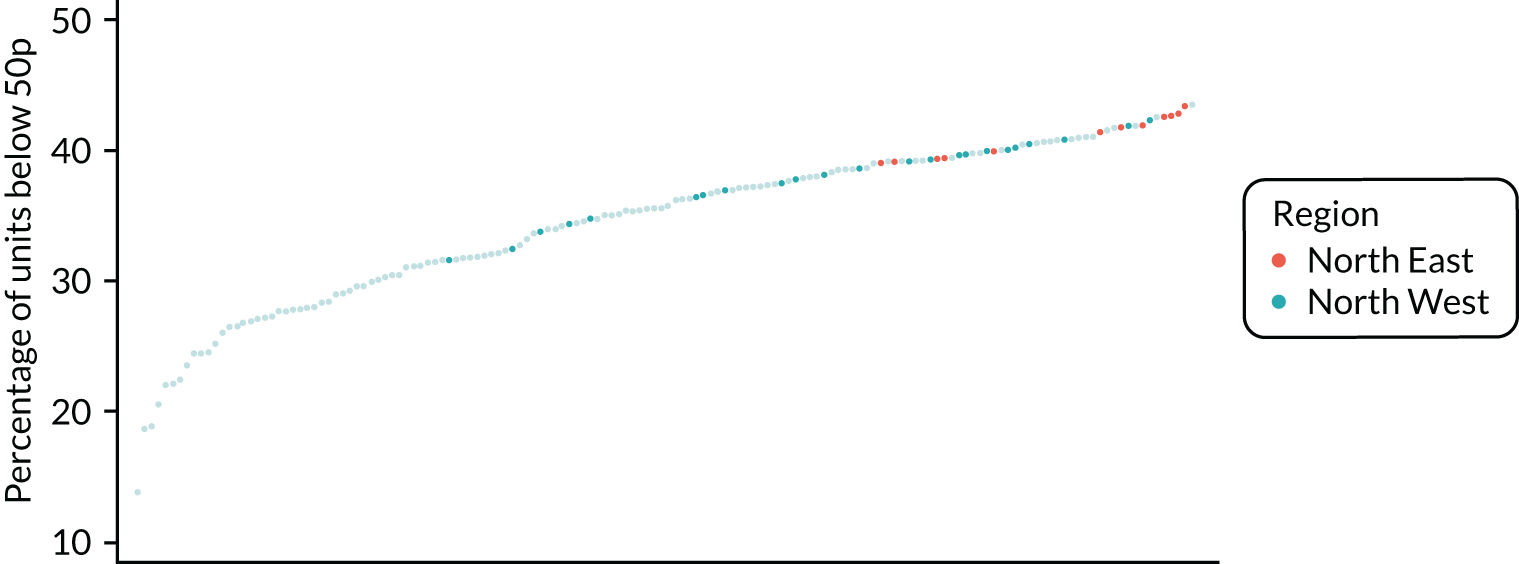
Figure 8 shows the variation in the percentage of units purchased at < 50p in the calibrated estimates. It shows that there remains substantial variation across UTLAs.
FIGURE 8.
Calibrated price distributions.
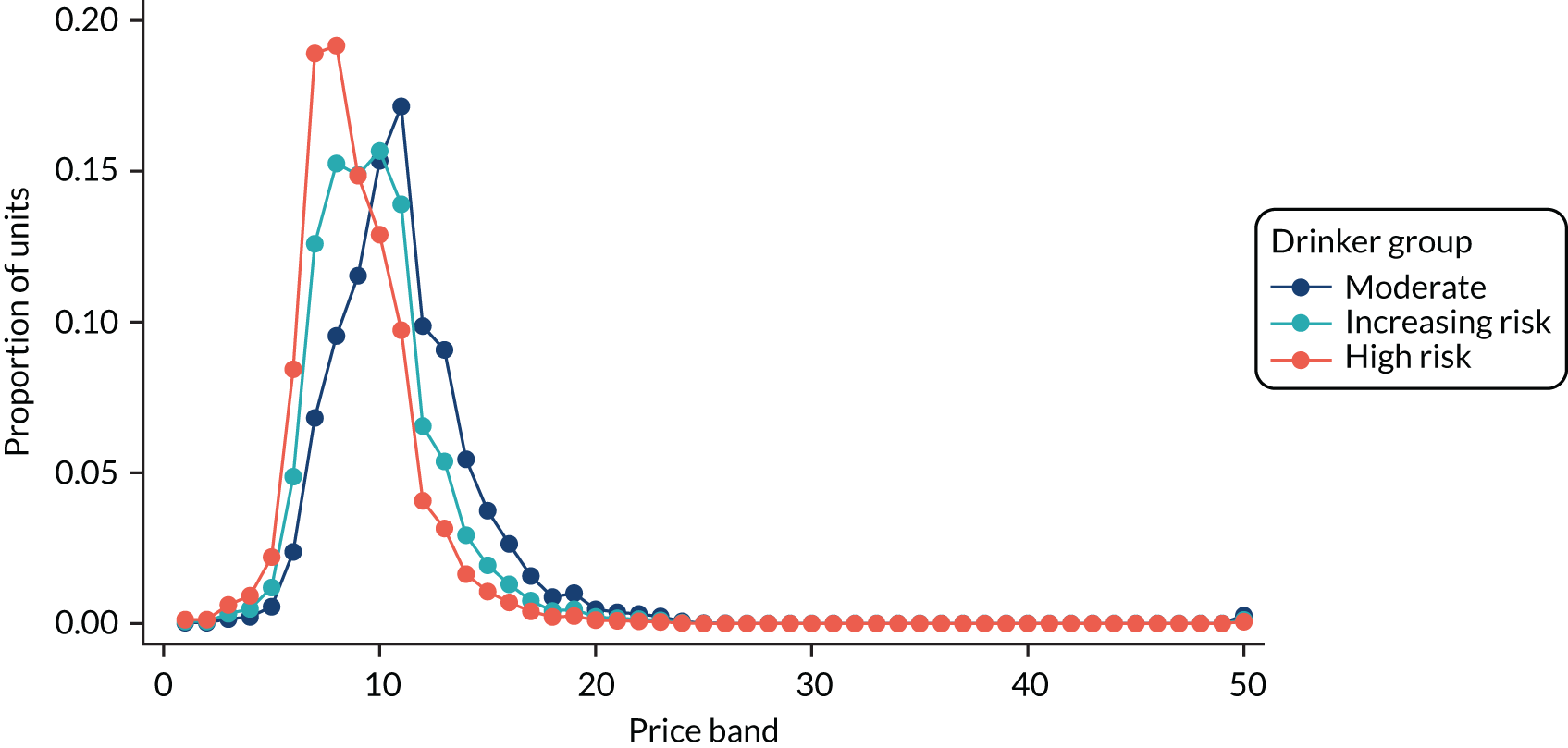
A further example of price distributions is shown in Figure 9, which shows the price distributions for a male, aged 35–54 years, in IMD quintile 3, for off-trade beer in Sefton. The lines show different distributions for moderate, increasing-risk and high-risk drinkers in this subgroup. The reason for showing this distribution is to give an idea of the granularity of the estimates. These graphs could be replicated for any subgroup of the population.
FIGURE 9.
Example price distributions: males, aged 35–54 years, IMD quintile 3, for off-trade beer in Sefton, split by moderate, increasing-risk and high-risk drinkers. The price bands are equal-width, 5p bands; the lowest band is ‘< £0.05 per unit’ and the top band is ‘≥ £2.45 per unit.
Results: preferences
Figure 10 shows how preferences vary across England by GOR, whereby the top of the band represents the GOR with the highest proportion of alcohol coming from that beverage type and the bottom of the band represents the GOR with the lowest proportion of alcohol coming from that beverage type. The North West region is coloured turquoise and is in the middle of the rankings by GOR.
FIGURE 10.
Preferences by GOR.
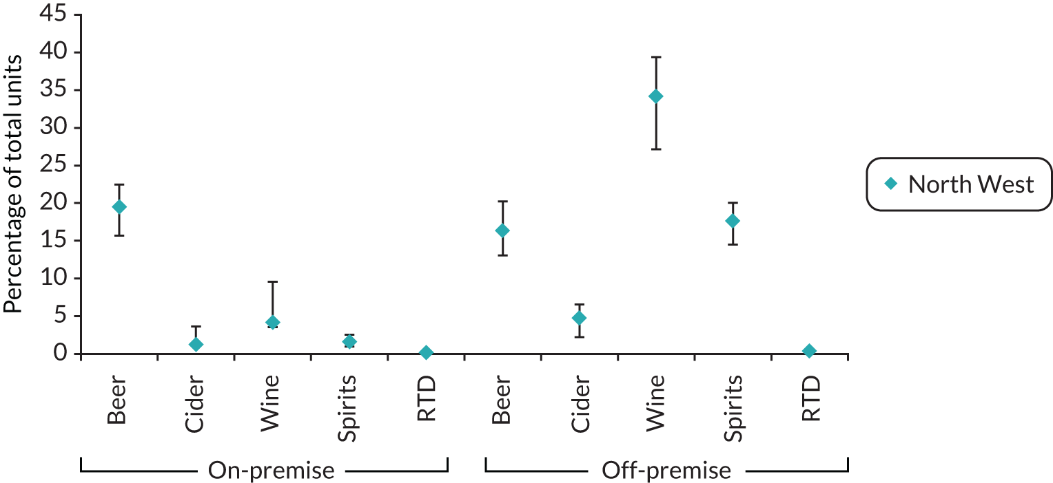
Similar to the price distributions, a graph like Figure 10 could be drawn for any subgroup.
An example of the detailed breakdown for preferences by subgroup is provided in Table 4.
| Alcohol category | Units (%) |
|---|---|
| On-premise | |
| Beer | 34.57 |
| Cider | 1.82 |
| Wine | 6.32 |
| Spirits | 1.61 |
| RTDs | 0.17 |
| Off-premise | |
| Beer | 23.18 |
| Cider | 5.03 |
| Wine | 20.94 |
| Spirits | 6.15 |
| RTDs | 0.20 |
Details on the Sheffield Alcohol Policy Model version 4.0: updates and revisions to the model to incorporate and model local authority data
Overview of Sheffield Alcohol Policy Model version 4.0
The aim of the SAPM version 4.0 is to appraise alcohol policy options via cost-effectiveness and cost–benefit analyses. This is achieved by breaking the policy impact into a series of linked effects to model the effects of:
-
the policy on the distribution of prices for different types of alcohol
-
changes in price distributions on patterns of both on-trade and off-trade alcohol consumption
-
changes in alcohol consumption patterns on consumer spending on alcohol
-
changes in alcohol consumption patterns on retailer and exchequer revenue from alcohol sales
-
changes in alcohol consumption patterns on levels of alcohol-related health harms
-
changes in alcohol consumption patterns on levels of alcohol-related crime.
To estimate the range of these effects, the SAPM version 4.0 consists of two connected models:
-
A model of the relationship between alcohol policies and alcohol consumption that accounts for the relationship between average weekly alcohol consumption, the patterns in which that alcohol is drunk and how these are distributed within the population considering gender, age, income/socioeconomic status and consumption level.
-
A model of the relationship between: (1) both average level and patterns of alcohol consumption and (2) harms related to health and workplace absenteeism and the costs associated with these harms.
Details on the modelling are also available in previously published works. 45–47
Baseline data for modelling the relationship between minimum unit pricing policy and alcohol consumption
As described in Estimating alcohol consumption for each local authority by population subgroup, alcohol consumption data are derived from the HSE, using a novel statistical modelling approach to adjust the original data to be representative of each UTLA in England. Unlike previous versions of the SAPM, we do not use the beverage-specific consumption information for each HSE individual, as the re-weighting procedure described in Estimating alcohol consumption for each local authority by population subgroup accounts for total alcohol consumption only. Therefore, these data take the form of individual-level data describing the demographic characteristics of each individual (age, sex, IMD quintile, mean alcohol consumption, peak alcohol consumption in the preceding week) and a weight that represents the number of individuals in the UTLA that they represent (i.e. the sum of the weights in each UTLA model is equal to the adult population).
As described in Methods for statistical modelling to estimate price distributions, pricing data are derived from the LCFS, using a variation on the same approach as that used for the consumption data. In previous national analysis versions of the SAPM, we have directly used transaction-level data from the LCFS. We do not have transaction-level data at UTLA level. Therefore, in this version, we use the statistical modelling described in Methods for statistical modelling to estimate price distributions to derive a data table. This data table takes the form of 60,000 rows of data, one for each unique combination of age (18–24, 25–34, 35–54 and ≥ 55 years), sex, IMD quintile, alcohol consumption category (moderate, increasing risk, high risk), drink type (beer, cider, wine, spirits and RTDs), purchase location (on- or off-trade) and price band (50 bands from 0–5p per unit to ≥ £2.45 per unit). For each row, the statistical models described in Estimating beverage preferences and the distribution of prices paid for each local authority by beverage category and population subgroup are used to derive the predicted probability that a unit of alcohol purchased by somebody of the relevant age, sex, IMD and drinker group characteristics will be that type of alcohol, in that setting and at that price.
The final data used are the population structure of each UTLA, taken from ONS mid-year population estimates. These are used to derive the population count by age, sex, IMD quintile and single year of age for each UTLA.
Modelling the impact of minimum unit pricing on prices
For each of the 10 types of alcohol included in the SAPM (five beverage types by two purchase locations), the first step in the modelling process is to estimate the impact of a price-based intervention, such as a MUP, on the price distribution at which alcohol can be purchased.
In line with previous iterations of the SAPM, we make the assumption that all prices below the MUP threshold are raised to the level of the threshold, whereas prices above the threshold are unaffected. This is operationalised in the model by reducing the probabilities of purchasing all types of alcohol at prices of < 50p to zero, and increasing the probabilities of purchasing the same types of alcohol at prices of 50–55p by the same amount. This assumption is highly likely to be conservative, as it is likely that, in reality, the supply-side response to a MUP policy would be to increase the prices of some items beyond the threshold, while also increasing the prices of other products that are not currently being sold below the threshold in order to maintain some degree of price differentiation. As a result, the observed price changes are likely to exceed those modelled here, with correspondingly larger reductions in consumption and impacts on model outcomes, such as reductions in the numbers of deaths, hospital admissions and crimes.
Modelling the impact of price changes on consumption
For each of the 10 types of alcohol, we calculated the mean price paid by each of the 120 age–sex–IMD–drinker subgroups in the model before and after the intervention. This gave us 1200 individual changes in price following the introduction of a MUP. The 10 price changes for each subgroup are combined with a 10 × 10 matrix of price elasticities (Table 5), which contains the own- and cross-price elasticities for each beverage type taken from a previously published and used study of price elasticities by Meng et al. 48 For each of the 120 subgroups, the 10 price changes are combined with these elasticities to estimate the percentage change in consumption of each beverage, using the following equation:
where:
-
%ΔCi is the estimated percentage change in consumption for beverage i
-
eii is the own-price elasticity for beverage i
-
%Δpi is the percentage change in price for beverage i
-
eij is the cross-price elasticities for the consumption of beverage i due to a change in the price of beverage j
-
%Δpj is the percentage change in price for beverage j.
| Purchase | |||||||||||
|---|---|---|---|---|---|---|---|---|---|---|---|
| Off-trade | On-trade | ||||||||||
| Beer | Cider | Wine | Spirits | RTDs | Beer | Cider | Wine | Spirits | RTDs | ||
| Price | Off-trade | ||||||||||
| Beer | –0.980* | –0.189 | 0.096 | –0.368 | –1.092 | –0.016 | –0.050 | 0.253 | 0.030 | 0.503 | |
| Cider | 0.065 | –1.268* | 0.118 | –0.122 | –0.239 | –0.053 | 0.093 | 0.067 | –0.108 | –0.194 | |
| Wine | –0.040 | 0.736* | –0.384* | 0.363 | 0.039 | –0.245 | –0.155 | 0.043 | –0.186 | 0.110 | |
| Spirits | 0.113 | –0.024 | 0.163 | –0.082 | –0.042 | 0.167 | 0.406 | 0.005 | 0.084 | 0.233 | |
| RTDs | –0.047 | –0.159 | –0.006 | 0.079 | –0.585* | –0.061 | 0.067 | 0.068 | –0.179* | 0.093 | |
| On-trade | |||||||||||
| Beer | 0.148 | –0.285 | 0.115 | –0.028 | 0.803 | –0.786* | 0.867 | 1.042* | 1.169* | –0.117 | |
| Cider | –0.100 | 0.071 | 0.043 | 0.021 | 0.365 | 0.035 | –0.591* | 0.072 | 0.237* | 0.241 | |
| Wine | –0.197 | 0.094 | –0.154 | –0.031 | –0.093 | –0.276 | –0.031 | –0.871* | –0.021 | –0.363 | |
| Spirits | 0.019 | –0.117 | –0.027 | –0.280 | –0.145 | –0.002 | –0.284 | 0.109 | –0.890* | 0.809* | |
| RTDs | 0.079 | 0.005 | –0.085 | –0.047 | 0.369 | 0.121 | –0.394 | –0.027 | –0.071 | –0.187 | |
For each subgroup, the cumulative probability of any unit purchased falling into each of the 10 categories was calculated and applied to the baseline consumption of each individual in the model to calculate the baseline weekly consumption of each beverage type. This was then adjusted using the percentage changes calculated using Equation 1 to obtain the estimated post-intervention consumption for each individual.
Model structure for modelling the relationship between consumption and harm
An epidemiological approach was used to model the relationship between consumption and harm, relating changes in alcohol consumption to changes in the risk of experiencing harmful outcomes. Risk functions relating consumption (however described) to level of risk are a fundamental component of the model.
The ‘consumption to harm’ model considers the impact of consumption on harms in two domains: health (including the impact on both mortality and morbidity) and crime.
In the following sections, we describe how the health component of the model estimates the impact of changes in alcohol consumption on 45 different health conditions, and how the crime component of the model estimates the impact on 14 different categories of offence. Both components use the same basic approach: the potential impact fraction (PIF).
The potential impact fraction methodology
The methodology is similar to that used in Gunning-Schepers’ Prevent model,49 being based on the notion of the alcohol-attributable fraction (AAF) and its more general form, the PIF.
The AAF of a disease can be defined as the difference between the overall average risk (or incidence rate) of the disease in the entire population (drinkers and never-drinkers) and the average risk in those without the exposure factor under investigation (never-drinkers), expressed as a fraction of the overall average risk. For example, the AAF for female breast cancer is simply the risk of breast cancer in the total female population minus the risk of breast cancer in women who have never consumed alcohol, divided by the breast cancer risk for the total female population. Thus, AAFs are used as a measure of the proportion of the disease that is attributable to alcohol. Although this approach has traditionally been used for chronic health-related outcomes, it can, in principle, be applied to other harms (including those outside the health domain).
The AAF can be calculated using the following formula:
where:
-
RRi is the relative risk due to exposure to alcohol at consumption state i
-
pi is the proportion of the population exposed to alcohol at consumption state i
-
n is the number of consumption states.
If the reference category is abstention from alcohol, then the AAF describes the proportion of outcomes that would not have occurred if everyone in the population had abstained from drinking. Thus, the numerator is essentially the excess expected cases due to alcohol exposure and the denominator is the total expected cases. In situations in which certain levels of alcohol consumption reduce the risk of an outcome (e.g. coronary heart disease), the AAF can be negative and would describe the additional cases that would have occurred if everyone were an abstainer.
Note that there are methodological difficulties with AAF studies. One problem is in defining the non-exposed group: in one sense ‘never-drinkers’ are the only correct non-exposed group, but they are rare and usually quite different from the general population in various respects. However, current non-drinkers include those who were heavy drinkers in the past (and these remain a high-risk group, especially if they have given up because of alcohol-related health problems). Several studies show that findings of avoided coronary heart disease risk may be based on systematic errors in the way abstainers were defined in the underlying studies. 50
The PIF is a generalisation of the AAF based on arbitrary changes to the prevalence of alcohol consumption (rather than assuming that all drinkers become abstainers). Note that a lag may exist between the exposure to alcohol and the resulting change in risk. The PIF can be calculated using the following formula:
where pi¯ is the modified prevalence for consumption state i, and state 0 corresponds to abstention.
In the model, alcohol consumption in a population subgroup is described non-parametrically by the associated observations from the HSE. For any harmful outcome, risk levels are associated with consumption level for each of the observations (note that these are not person-level risk functions). The associated prevalence for the observation is simply defined by its sample weight from the survey. Therefore, the PIF is implemented in the model as:
where:
-
wi is the weight for observation i
-
RRi¯ is the modified risk for the new consumption level
-
N is the number of samples.
Applying potential impact fractions for health outcomes
The impact of changes in alcohol consumption on health harms was examined using three different implementations of the PIF, depending on the health condition type:
-
direct application of consumption measures to calculate PIFs for wholly attributable acute and chronic conditions
-
relative risk functions from the published literature for partial chronic conditions
-
occasion-level relative risk functions from the published literature converted to annualised risks for partially attributable acute conditions (i.e. injuries).
Wholly attributable conditions
As wholly attributable chronic and acute conditions, by definition, have an AAF of 1 and, therefore, the relative risk cannot be defined, the relative risk term in Equation 7 is replaced with alcohol consumption that is likely to lead to increased risk for the health condition, denoted by RiskAlci, in the revised Equation 8:
For wholly attributable chronic conditions, RiskAlci is defined as the difference between mean daily consumption and a lower threshold below which risk is assumed to be equivalent to that of abstainers. In line with previous studies, these thresholds were assumed to be four and three units per day for men and women, respectively. 51 Below these thresholds, RiskAlci is assumed to be 0. An equivalent approach is used for wholly attributable acute conditions, for which RiskAlci is defined as the difference between peak day consumption (the response that individual HSE respondents give to the question ‘on the day in the last week when you drank the most, how much did you drink?’) and the cut-off thresholds of four/three units for men/women at which we assume the acute risk starts to increase, or 0 if peak day consumption is below the threshold.
Partially attributable chronic conditions
The relative risk functions for all chronic conditions that are partially attributable to alcohol are taken from published meta-analyses and are used in Equation 7. The sources for these risk functions and their corresponding curves are illustrated in Angus et al. 52
Ischaemic heart disease represents a special case in SAPM version 4.0 as this is the only condition for which a literature-based risk function is adjusted to reflect additional evidence. Although many studies have found that drinking at low levels reduces the risk of ischaemic heart disease relative to abstainers,53 it has been demonstrated that this reduced risk is substantially attenuated or eliminated for those engaging in heavy episodic drinking (defined as consuming at least 7.5 units on a single day) at least once a month. 54 In the SAPM, this evidence is incorporated using a method employed by Shield et al. ,55 whereby any protective effect is removed (i.e. the relative risk is assumed to be at least 1) for any drinkers who consume > 7.5 units per day, on average (52.5 units per week). This limited adjustment means that cardioprotective effects are likely to be overestimated in the model, as many individuals with a mean consumption of < 7.5 units per day probably drink this amount at least once a month. The most recent epidemiological risk functions for mortality suggest that protective effects disappear at below 7.5 units per day56 and, therefore, this adjustment has no effect. However, the evidence for morbidity outcomes is older and suggests that protective effects exist above a mean consumption level of 7.5 units per day;53 these are therefore removed in line with the newer evidence on heavy episodic drinking.
Partially attributable acute conditions
Partially attributable acute conditions include various traffic and non-traffic injuries. The identified relative risk functions for these conditions57 are different from the relative risk functions for partially attributable chronic conditions and cannot be used directly in Equation 4. The input and outcome of the relative risk functions for partially attributable chronic conditions are usual alcohol consumption and relative risk over a certain period of time, respectively; however, the input and outcome of the identified relative risk functions for traffic and non-traffic injuries are levels of drinking on the occasion prior to the injury and the relative risk for the drinking occasion, respectively. 58 As the SAPM version 4.0 works on annual cycles, relative risk in Equation 7 is defined as annual relative risk. Therefore, to apply Equation 7, single drinking occasion-based relative risk needs to be converted to long-term (e.g. annual) relative risk of an individual in the survey.
A method to estimate annualised relative risk of alcohol-attributable traffic- and non-traffic injuries has been developed. A detailed description of the method can be found elsewhere. 59,60 Briefly, three measures are defined to represent drinking pattern based on single drinking occasions, which are the frequency of drinking occasions (defined as n, or number of drinking occasions per week), the mean level of alcohol consumption for a given drinking occasion (defined as µ, or units of alcohol) and the variability of alcohol consumption for a given drinking occasion (defined as σ, or standard deviation of units of alcohol consumed on drinking occasions). Using the ONS National Diet and Nutrition Survey,60 regression models were fitted to relate the three measures with mean consumption and a range of independent variables (e.g. age, gender, education and ethnicity). These regression models are used to impute the three measures for each individual in the HSE. For each individual, alcohol consumption on a given drinking occasion is assumed to follow a normal distribution, with mean of µ and standard deviation of σ; and the duration of intoxication for a given drinking occasion is calculated by applying the equation for estimating blood alcohol content. Finally, a series of integrations were performed to calculate the annualised relative risk for traffic and non-traffic accidents.
The annualised relative risk obtained from this calculation process is used in Equation 7 to estimate the PIF for partially attributable acute conditions.
Conditions defined in the ICD-10
Table 6 lists the conditions that are in the SAPM version 4.0 that are defined in the ICD-10.
| Condition | ICD-10 code(s) | Condition type |
|---|---|---|
| Oropharyngeal cancer | C00–06, C09–10, C12–C14 | Partial chronic |
| Oesophageal cancer | C15 | Partial chronic |
| Colorectal cancer | C18–C20 | Partial chronic |
| Cancer of the liver and intrahepatic bile ducts | C22 | Partial chronic |
| Pancreatic cancer | C25 | Partial chronic |
| Laryngeal cancer | C32 | Partial chronic |
| Breast cancer | C50 | Partial chronic |
| Hypertensive diseases | I10–I14 | Partial chronic |
| Ischaemic heart disease | I20–I25 | Partial chronic |
| Alcoholic cardiomyopathy | I42.6 | 100% chronic |
| Cardiac arrhythmias | I47–I49 | Partial chronic |
| Haemorrhagic stroke | I60–I62 | Partial chronic |
| Ischaemic stroke | I63–I67 | Partial chronic |
| Cirrhosis of the liver (excluding alcoholic liver disease) | K70 (excluding K70.0–K70.4, K70.9), K73–K74 | Partial chronic |
| Alcoholic gastritis | K29.2 | 100% chronic |
| Alcoholic liver disease | K70.0–K70.4, K70.9 | 100% chronic |
| Acute pancreatitis (alcohol induced) | K85.2 | 100% chronic |
| Acute pancreatitis | K85 (excluding K85.2, K85.3) | Partial chronic |
| Chronic pancreatitis (alcohol induced) | K86.0 | 100% chronic |
| Chronic pancreatitis | K86 (excluding K86.0) | Partial chronic |
| Excessive blood level of alcohol | R78.0 | 100% acute |
| Toxic effect of alcohol | T51.0, T51.1, T51.8, T51.9 | 100% acute |
| Accidental poisoning by exposure to noxious substances | X40–X49 (excluding X45), Y10–Y14, Y16–Y19, T36–T50, T52–T65 | Partial acute |
| Alcohol poisoning | X45, X65, Y15 | 100% acute |
| Evidence of alcohol involvement determined by blood alcohol level | Y90 | 100% acute |
| Transport injuries (including road traffic accidents) | V01–V98, Y85.0 | Partial acute |
| Fall injuries | W00–W19 | Partial acute |
| Exposure to mechanical forces (including machinery accidents) | W20–W52 | Partial acute |
| Drowning | W65–W74, Y21 | Partial acute |
| Fire injuries | X00–X09, Y26 | Partial acute |
| Other unintentional injuries | W75–W99, X10–X33, Y20, Y22–Y25, Y27–Y29, Y31–Y34 | Partial acute |
| Intentional self-harm | X60–X84 (excluding X65), Y87.0 | Partial acute |
| Assault | X85–Y09, Y87.1 | Partial acute |
| Other intentional injuries | Y35 | Partial acute |
| Diabetes (type 2) | E11 | Partial chronic |
| Alcohol-induced pseudo-Cushing syndrome | E24.4 | 100% chronic |
| Acute intoxication | F10.0 | 100% acute |
| Mental and behavioural disorders due to use of alcohol | F10.1–F10.9 | 100% chronic |
| Degeneration | G31.2 | 100% chronic |
| Epilepsy and status epilepticus | G40–G41 | Partial chronic |
| Alcoholic polyneuropathy | G62.1 | 100% chronic |
| Alcoholic myopathy | G72.1 | 100% chronic |
| Maternal care for (suspected) damage to fetus from alcohol | O35.4 | 100% chronic |
| Tuberculosis | A15–A19 | Partial chronic |
| Lower respiratory tract infections | J09–J18 | Partial chronic |
Mortality data
For each of the 45 health conditions listed in Table 6, we obtained mortality counts, further stratified by age (four categories: 18–24, 25–34, 35–54 and 55–89 years), sex and socioeconomic status (five quintiles of the IMD based on the deceased’s home postcode), for every one of the 151 UTLAs in England from the ONS. To address year-on-year variance in small counts, we pooled data across the years 2012–16 and converted to mortality rates per 100,000, using population estimates for the relevant years from the ONS. 61
Hospitalisation data
For each of the 45 health conditions listed in Table 6, we calculated admission rates, stratified by age, sex, socioeconomic status and UTLA, from individual patient records taken from HES data for England. As each individual admission can have multiple ICD-10 diagnostic codes, each admission was coded to a single condition using the ‘broad measure’ approach, which is recommended by Public Health England (PHE) as the most appropriate measure ‘of the total burden that alcohol has on community and health services’62 (contains public sector information licensed under the Open Government Licence v3.0). To prevent double-counting, admissions within 1 year for the same individual were linked; if there were multiple admissions coded to different conditions in a single year, only the admissions for one condition were retained. For a full description of this process, see Jones et al. 63 From this process, two outcomes were produced:
-
Morbidity rates per 100,000 (derived using ONS population estimates) for each health condition and age–sex–socioeconomic status subgroup, after removing all repeat admissions. That is, these rates represent the rate of individuals with each condition in each subgroup. As with the mortality data, year-on-year variance in small counts was addressed by calculating rates based on pooled data for 2012/13–2016/17.
-
The average number of admissions per year for somebody with at least one admission by condition and age group. These figures were used to estimate the number of hospital admissions that were associated with the modelled morbidity prevalence and changes in this prevalence.
Mortality model structure
A simplified version of the model structure for mortality is presented in Figure 11. The model is developed to represent the population of England in a life table. Separate life tables have been implemented for males and females.
FIGURE 11.
Simplified mortality model structure.
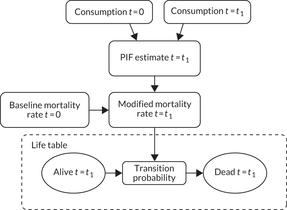
The life table is implemented as a linked set of simple Markov models with individuals of age a transitioning between two states – alive or dead – at model time step t. A Markov model is a state-transition model in which individuals can exist in a set number of states at any time period and transition between states using a set of transition probabilities, which are conditional on the current state of the individual. Those of age a still alive after the transition then form the initial population for age a + 1 at time t + 1, and the sequence repeats.
The transition probabilities from the alive to dead state are broken down by condition and are individually modified via PIFs over time t, where the PIF essentially varies with consumption over time:
where:
-
PIFt is the PIF relating to consumption at time t
-
i = survey sample number
-
N = number of samples in subgroup i
-
RRi,t is the risk relating to the consumption of SHeS sample i at time t
-
RRi,0 is the risk at baseline
-
wi is the weight of sample i.
Note that the PIF can be decomposed to enable different population groups at baseline (e.g. moderate, increasing-risk and high-risk drinkers or individuals in poverty and not in poverty) to be followed separately over the course of the model.
The model computes mortality results for two scenarios (a baseline – implemented as ‘no change to consumption’ in the analysis herein – and an intervention). The effect of the intervention is then calculated as the difference between the life table for the intervention scenario and the life table for the baseline scenario, enabling the change in the total expected deaths attributable to alcohol as a result of the policy to be estimated.
Outcomes from mortality modelling are expressed in terms of life-years saved. Morbidity valuation is the purpose of a second model described below.
Morbidity model structure
A simplified schematic of the morbidity model is shown in Figure 12. The model focuses on the expected disease prevalence for population cohorts. Note that if an incidence-based approach were used instead, then much more detailed modelling of survival time, cure rates, death rates and, possibly, disease progression for each disease for each population subgroup would be required.
FIGURE 12.
Simplified morbidity model structure. QALY, quality-adjusted life-year.
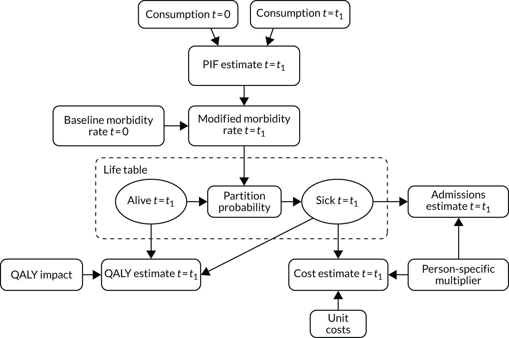
The morbidity model works by partitioning the alive population at time t, rather than using a transition approach between states, as previously described for the mortality model. Alive individuals are partitioned between all 45 alcohol-related conditions (and a 46th condition representing overall population health, not attributable to alcohol).
As in the mortality model, the PIF is calculated based on the consumption distribution at times 0 and t. The PIF is then used to modify the partition rate (i.e. the distribution of the 45 conditions for alive individuals) to produce person-specific sickness volumes. These volumes form the basis for estimating both health service costs and health-related quality of life.
Time lag effects for chronic harms
When modelling the link between consumption and harm, one important input is the assumption surrounding the ‘time lag’: the time needed to achieve the full benefit (reduction in harms) associated with a reduction in consumption. Such data are necessary for chronic conditions whereby the development of diseases often occurs over many years.
Following a 2012 systematic review,64 the SAPM version 4.0 incorporates lag structures for all chronic harms based on the best available published evidence to estimate the temporal relationship between changes in consumption and changes in risk of harm (see table 2 in Holmes et al. 64 for full details of these relationships as implemented in the model). In line with the findings of this review, health outcomes are reported at 20 years as ‘full effect’, as this is the time at which the full impact of a change in consumption on health will have occurred. Note that this 20-year time horizon for the model means that all outcomes are reported over the 20 years subsequent to the model baseline year (2017).
NHS costs used
Estimates of the costs associated with morbidity for each health condition were taken from previously published estimates of the full NHS cost of each condition,51 inflated to 2017 prices using the Hospital and Community Health Service index. 65 The final costs used in the models are presented in Table 7.
| Health condition | Annual NHS cost (£) |
|---|---|
| Oropharyngeal cancer | 9828 |
| Oesophageal cancer | 10,106 |
| Colorectal cancer | 8414 |
| Cancer of the liver and intrahepatic bile ducts | 6749 |
| Pancreatic cancer | 8824 |
| Laryngeal cancer | 5405 |
| Breast cancer | 14,655 |
| Hypertensive diseases | 5442 |
| Ischaemic heart disease | 8511 |
| Alcoholic cardiomyopathy | 5830 |
| Cardiac arrhythmias | 22,731 |
| Haemorrhagic stroke | 7243 |
| Ischaemic stroke | 5830 |
| Cirrhosis of the liver (excluding alcoholic liver disease) | 8511 |
| Alcoholic gastritis | 6333 |
| Alcoholic liver disease | 8511 |
| Acute pancreatitis (alcohol induced) | 8511 |
| Acute pancreatitis | 8511 |
| Chronic pancreatitis (alcohol induced) | 17,126 |
| Chronic pancreatitis | 5005 |
| Excessive blood level of alcohol | 6167 |
| Toxic effect of alcohol | 3550 |
| Accidental poisoning by exposure to noxious substances | 10,430 |
| Alcohol poisoning | 4287 |
| Evidence of alcohol involvement determined by blood alcohol level | 4287 |
| Transport injuries (including road traffic accidents) | 4966 |
| Fall injuries | 5369 |
| Exposure to mechanical forces (including machinery accidents) | 8511 |
| Drowning | 6207 |
| Fire injuries | 6828 |
| Other unintentional injuries | 6990 |
| Intentional self-harm | 6990 |
| Assault | 19,868 |
| Other intentional injuries | 7422 |
| Diabetes (type 2) | 9221 |
| Alcohol-induced pseudo-Cushing syndrome | 12,381 |
| Acute intoxication | 15,281 |
| Mental and behavioural disorders due to use of alcohol | 8511 |
| Degeneration | 8511 |
| Epilepsy and status epilepticus | 8511 |
| Alcoholic polyneuropathy | 7865 |
| Alcoholic myopathy | 6983 |
| Maternal care for (suspected) damage to fetus from alcohol | 5286 |
| Tuberculosis | 5899 |
| Lower respiratory tract infections | 5378 |
Data and methods used to model crime
Crime model structure
The structure of the crime model is similar to the approach used in the health model. We assume that risks of committing a criminal offence are associated with intoxication, rather than chronic consumption; therefore, risk is modelled as a function of peak day consumption. For each offence category included in the model, published estimates of the proportion of such offences that were attributable to alcohol (the AAF) were obtained (see table 2.3 in Purshouse et al. 51). As for health harms, a lower threshold of four/three units per day for men/women, respectively, is used, below which the risk is assumed to be equivalent to that of a non-drinker. Above these thresholds, risk is assumed to rise linearly with consumption, meaning that the relative risk of committing an offence can be written as:
where i represents peak day consumption, T represents the threshold and β is a slope parameter.
For each age–gender subgroup in the model, Equation 10 is combined with Equation 7 and the existing AAFs to calibrate the value of the slope parameter β to give the correct AAF value. Having ascertained the correct value of β, the PIF approach can then be used, as for partially alcohol-attributable chronic conditions, using the formula for relative risk set out in Equation 10. We assume that there is no time delay between changes in consumption due to the implementation of a MUP and the risk of crime outcomes occurring. So, ‘full effect’ is assumed to occur in the first year after policy implementation. In other words, the crime model does not include any equivalent of the lag effects that we model for chronic diseases in the health model.
Source of data on reported crimes
The key data source for baseline crime volumes is police-recorded crime statistics from the ONS for the years March 2003–March 2017. The raw data, separated by police force area, were downloaded from the ONS police-recorded crime statistics and we used the number of headline offences (see table C3: Community Safety Partnerships: Number of recorded crimes for headline offences, year ending March 201766,67). The average yearly counts for each of the offences were calculated across the 14-year period to minimise sampling error, particularly for offences that are relatively scarce, such as homicide. Data were available at lower-tier local authority level, and these were mapped onto the UTLAs used in the modelling, using the mapping set out in Table 8.
| UTLA | Police force area | Lower-tier local authority |
|---|---|---|
| Blackburn | Lancashire | Blackburn with Darwen |
| Blackpool | Lancashire | Blackpool |
| Bolton | Greater Manchester | Bolton |
| Bury | Greater Manchester | Bury |
| Cheshire East | Cheshire | Cheshire East |
| Cheshire West and Chester | Cheshire | Cheshire West and Chester |
| Cumbria | Cumbria | Sum of all local authority in Cumbria |
| Halton | Cheshire | Halton |
| Knowsley | Merseyside | Knowsley |
| Lancashire | Lancashire total | Sum of all local authority in Lancashire, minus Blackburn and Blackpool |
| Liverpool | Merseyside | Liverpool |
| Manchester | Greater Manchester | Manchester |
| Oldham | Greater Manchester | Oldham |
| Rochdale | Greater Manchester | Rochdale |
| Salford | Greater Manchester | Salford |
| Sefton | Merseyside | Sefton |
| St Helens | Merseyside | St Helens |
| Stockport | Greater Manchester | Stockport |
| Trafford | Greater Manchester | Trafford |
| Tameside | Greater Manchester | Tameside |
| Wigan | Greater Manchester | Wigan |
| Wirral | Merseyside | Wirral |
| Warrington | Cheshire | Warrington |
Categories of crime used
Fourteen separate offence categories, as set out in the recorded crime data, are included in the modelling: homicide, violence with injury, violence without injury, sexual offences, robbery, residential burglary, non-domestic burglary, vehicle offences, theft from the person, bicycle theft, shoplifting, other theft offences, criminal damage and arson, and public order offences.
Multipliers for unrecorded crime
It is well known that not all crimes are reported and the model accounts for this. The UK Home Office has produced estimates of the number of offences that occur for every recorded offence, and these ‘multipliers’ are used to adjust the baseline recorded crime data to estimate the true baseline rates of each offence. 68
Splitting crimes by age and sex
Recorded crime data record only the total volume of offences, with no detail on the characteristics of the offenders. As the SAPM requires age- and gender-specific baseline offence rates, we needed to use additional data on the distribution of offences across age and gender groups. These data come from previously published work for the National Institute for Health and Care Excellence (NICE) (see table A8.1 in Purshouse et al. 69) and give the proportion of offences committed by each age–gender group by offence category. These proportions are used to partition the baseline crime volumes into subgroup-specific rates.
Costs of crime
Estimates of the cost of crime to society come from a report produced by the UK Home Office in 2011. 68 This includes estimates of the direct costs to the criminal justice system of each offence committed, including costs associated with policing, prosecuting and incarcerating offenders, offset against any fines collected. The costs also include a financial valuation of the impact on health-related quality of life to victims, through both reduced quality and length of life. These costs were assigned to the 14 offence categories in the model and inflated to 2016 prices using the Retail Prices Index. 70
Time horizon and discounting
In view of evidence suggesting that there may be a lag of up to 20 years between changes in alcohol consumption and changes in the risk of health harms,64 the time horizon of the model is 20 years. This allows the results presented to reflect the full effect of the policy on health outcomes. In line with the NICE guidelines on economic evaluations,71 all costs are discounted at 3.5%.
The detailed analysis plan
The assumptions on the impact of a minimum unit price intervention on the price distributions
We assume that prices of products currently sold at < 50p per unit rise to exactly 50p per unit. We assume that other prices remain unchanged.
Geographies analysed
We used the UTLA-level data described previously to produce the SAPMLA versions for each UTLA in the North West (23 UTLAs) and North East (12 UTLAs) of England. The process used to generate UTLA-level inputs was repeated at GOR level, and these inputs were used to create further models for each of the nine GORs.
Analysis of local burden of harm (comparison of current harm versus estimated harm if there were zero alcohol consumption)
For each geography, the current level of harm that is attributable to alcohol is estimated by comparing the data on current total level of harm (due to alcohol and other causes) with the results of a model run assuming that the population stopped drinking entirely.
Appraising the impact of 30p, 40p, 50p, 60p and 70p per unit minimum unit pricing policies
The models were then used to appraise the impact of 30p, 40p, 50p, 60p and 70p per unit minimum unit pricing policies. Finally, results for the nine GORs were combined to estimate the overall impact of each policy at the national level. The outputs from each model were the changes in alcohol consumption, changes in spending on alcohol, resulting changes in revenue to retailers and the exchequer, changes in alcohol-related hospital admissions and deaths, reductions in NHS costs, changes in annual volumes of crime and the associated costs.
Analysis of the slope index of inequality
All outputs were stratified by drinker group (moderate, increasing risk and high risk) and IMD quintile. The slope index of inequality16 (a regression approach to estimate the absolute difference between the highest and lowest percentiles in the population) was calculated for alcohol-attributable mortality both before and after each policy.
Chapter 3 Results
This chapter consists of three sections. The first section is a summary of the comparative results for the local authorities across the North West region. The second and third sections show some of the detailed results available to specific UTLAs using examples of the ‘evidence assets’ that have been co-produced with stakeholders. Section 2 shows a high-level summary of the results on a two-sided A4 presentation for one local authority (Sefton). A similar two-sided A4 presentation is shown for the North West region as a whole. This exemplifies one way in which the material could be disseminated by a key contact in each local authority (e.g. the public health lead for alcohol) to key opinion leaders in their local authority and wider community. The third section shows some examples of the more detailed evidence assets. We have developed a PowerPoint slide deck that can ‘tell the story’ of one local authority, using 65 slide PowerPoint evidence assets. We present here some examples of the key slides and discuss the results for the Sefton local authority in the North West region. Slides similar to these were presented to the audiences that attended the two major stakeholder meetings in the North West and North East regions, held on 7 November 2018 and 21 November 2018, respectively.
Summary of the comparative results for the local authorities across the North West region
Table 9 shows that the current baseline estimated level of alcohol consumption and alcohol-related harm is higher in almost all of the North West UTLAs than the national average for England. Only 3 out of 23 local authorities had lower mean weekly alcohol consumption than the English average, and all 23 local authorities had a higher proportion of the population drinking at the high-risk level. For mortality, the annual alcohol-attributable death rate per 100,000 population varies substantially, with the highest (Blackpool) being just over twice as high as the lowest (Cumbria); all are higher than the national average. Summing the 23 local authorities gives an estimated total number of alcohol-attributable deaths of 1791 annually, which is slightly higher than when the model is run on the North West as a whole (1729 deaths). Similar patterns are seen for the alcohol-attributable hospitalisation rate per 100,000 population: the highest rate (Salford) is almost 50% higher than the lowest rate (Manchester), and there are a total of 108,403 alcohol-attributable hospitalisations per year for the North West region. The annual cost of alcohol-attributable diseases to the NHS varies from £10M to > £75M across the local authorities, with a regional total estimate of £504M. The alcohol-attributable crimes total for the North West is estimated at ≈ 340,000, and the crime rate per population also varied substantially, with the highest rate (Blackpool) being around double that of the lowest (Cheshire East).
| Data | North West UTLAs | North West | North East | National | ||||||||||||||||||||||
|---|---|---|---|---|---|---|---|---|---|---|---|---|---|---|---|---|---|---|---|---|---|---|---|---|---|---|
| Blackburn | Blackpool | Bolton | Bury | Cheshire East | Cheshire West | Cumbria | Halton | Knowsley | Lancashire | Liverpool | Manchester | Oldham | Rochdale | Salford | Sefton | St Helens | Stockport | Tameside | Trafford | Warrington | Wigan | Wirral | ||||
| Adult population (aged ≥ 18 years) (n) | 107,370 | 110,057 | 210,997 | 141,864 | 291,843 | 260,110 | 395,834 | 96,398 | 111,982 | 919,325 | 376,291 | 397,577 | 167,446 | 159,116 | 183,986 | 215,036 | 137,663 | 219,959 | 169,213 | 174,290 | 158,427 | 248,309 | 247,762 | 5,500,855 | 2,050,703 | 41,614,894 |
| Mean weekly alcohol consumption (units) | ||||||||||||||||||||||||||
| Per drinker | 14.3 | 14.2 | 14.3 | 14.6 | 14.5 | 14.3 | 14.3 | 14.9 | 14.7 | 14.2 | 14.4 | 14.6 | 14.3 | 14.5 | 14.8 | 13.9 | 14.7 | 14.3 | 14.5 | 13.9 | 14.3 | 14.7 | 14.5 | 14.4 | 16.4 | 13.3 |
| Moderate drinkers | 4.1 | 4.2 | 4.2 | 4.4 | 4.6 | 4.5 | 4.4 | 4.3 | 4.1 | 4.4 | 4.1 | 4.0 | 4.2 | 4.2 | 4.3 | 4.3 | 4.3 | 4.5 | 4.3 | 4.5 | 4.5 | 4.4 | 4.4 | 4.3 | 4.4 | 4.3 |
| Increasing-risk drinkers | 25.2 | 23.4 | 24.9 | 25.1 | 24.9 | 24.7 | 24.7 | 24.9 | 25.0 | 24.8 | 24.7 | 25.7 | 25.1 | 25.3 | 24.8 | 24.3 | 24.6 | 24.7 | 24.7 | 24.5 | 24.5 | 24.7 | 24.4 | 24.8 | 25.2 | 24.7 |
| High-risk drinkers | 80.0 | 86.6 | 77.8 | 75.1 | 72.7 | 74.1 | 75.6 | 78.8 | 79.5 | 75.7 | 82.0 | 80.6 | 77.4 | 79.1 | 80.4 | 77.0 | 79.3 | 75.5 | 80.1 | 74.0 | 75.8 | 77.8 | 78.1 | 77.5 | 79.0 | 75.6 |
| Abstaining (%) | 29.4 | 17.1 | 22.0 | 17.5 | 12.9 | 13.5 | 14.2 | 16.8 | 18.6 | 16.4 | 20.4 | 29.0 | 24.0 | 23.5 | 18.8 | 15.0 | 16.1 | 15.4 | 18.8 | 15.9 | 13.9 | 15.0 | 15.4 | 17.9 | 15.7 | 17.1 |
| Moderate drinkers (%) | 48.6 | 59.4 | 53.2 | 54.8 | 57.3 | 57.8 | 57.4 | 55.9 | 55.5 | 56.3 | 55.4 | 48.6 | 51.7 | 51.9 | 55.2 | 58.5 | 56.9 | 56.7 | 55.4 | 57.0 | 57.8 | 57.0 | 57.3 | 55.5 | 53.8 | 57.4 |
| Increasing-risk drinkers (%) | 17.4 | 17.6 | 19.8 | 22.5 | 24.4 | 23.4 | 23.1 | 21.4 | 20.0 | 22.1 | 18.7 | 17.6 | 19.4 | 19.5 | 20.2 | 21.2 | 21.2 | 22.5 | 20.2 | 22.1 | 22.9 | 22.3 | 21.5 | 21.2 | 23.4 | 21.0 |
| High-risk drinkers (%) | 4.7 | 5.9 | 5.1 | 5.3 | 5.4 | 5.3 | 5.4 | 6.0 | 5.9 | 5.2 | 5.5 | 4.8 | 4.9 | 5.1 | 5.8 | 5.3 | 5.8 | 5.4 | 5.5 | 5.0 | 5.4 | 5.7 | 5.8 | 5.3 | 7.1 | 4.5 |
| Alcohol-related deaths per year (n) | 32 | 56 | 67 | 45 | 80 | 75 | 96 | 32 | 42 | 254 | 146 | 115 | 54 | 55 | 60 | 79 | 53 | 67 | 56 | 49 | 46 | 87 | 84 | 1791 | 697 | 9862 |
| Alcohol-related mortality per 100,000 adult population | 29.4 | 50.6 | 32.0 | 32.0 | 27.3 | 28.7 | 24.2 | 33.4 | 37.7 | 27.7 | 38.7 | 28.8 | 32.1 | 34.7 | 32.6 | 36.5 | 38.7 | 30.5 | 33.0 | 28.2 | 29.2 | 35.0 | 33.8 | 32.6 | 34.0 | 23.7 |
| Alcohol-attributable admissions per year (n) | 2203 | 2633 | 3692 | 2495 | 5247 | 4515 | 7041 | 2152 | 2615 | 16,779 | 7881 | 6750 | 3055 | 3137 | 4610 | 4472 | 3167 | 4563 | 3649 | 3077 | 3024 | 5225 | 5842 | 108,403 | 41,159 | 650,879 |
| Alcohol-attributable admissions per 100,000 adult population | 2052.0 | 2392.4 | 1749.9 | 1758.8 | 1797.7 | 1735.8 | 1778.7 | 2232.5 | 2335.1 | 1825.2 | 2094.3 | 1697.9 | 1824.6 | 1971.3 | 2505.6 | 2079.6 | 2300.7 | 2074.5 | 2156.3 | 1765.3 | 1908.7 | 2104.4 | 2357.9 | 1970.7 | 2007.1 | 1563.0 |
| Alcohol-attributable crimes per year (n) | 7098 | 10,605 | 13,478 | 8385 | 13,771 | 14,869 | 22,547 | 6839 | 7005 | 50,507 | 27,196 | 31,422 | 10,989 | 12,249 | 13,110 | 10,762 | 8100 | 12,815 | 11,220 | 9282 | 8974 | 13,993 | 12,904 | 341,202 | 125,625 | 2,299,140 |
| Alcohol-attributable crimes per 100,000 adult population | 6610.4 | 9636.0 | 6387.6 | 5910.4 | 4718.8 | 5716.5 | 5696.0 | 7094.2 | 6255.5 | 5494.0 | 7227.4 | 7903.4 | 6562.8 | 7698.4 | 7125.3 | 5004.6 | 5883.8 | 5826.2 | 6630.7 | 5325.5 | 5664.5 | 5635.3 | 5208.4 | 6202.7 | 6125.9 | 5521.2 |
| Alcohol-attributable NHS cost per year (£000,000) | 10.4 | 12.8 | 17.0 | 11.4 | 23.1 | 20.3 | 31.0 | 10.0 | 12.2 | 75.4 | 38.3 | 33.2 | 14.3 | 14.7 | 23.3 | 20.4 | 14.9 | 20.9 | 17.1 | 14.1 | 14.0 | 23.8 | 27.6 | 504.6 | 185.5 | 2855.4 |
| Mean annual expenditure on alcohol (£) | ||||||||||||||||||||||||||
| Per adult | 436 | 477 | 474 | 514 | 556 | 538 | 515 | 506 | 480 | 507 | 471 | 452 | 463 | 467 | 497 | 494 | 501 | 527 | 483 | 528 | 530 | 518 | 508 | 500 | 570 | 481 |
| Moderate drinkers | 186 | 190 | 197 | 208 | 226 | 221 | 208 | 197 | 187 | 209 | 191 | 188 | 192 | 190 | 198 | 204 | 198 | 217 | 195 | 224 | 218 | 204 | 204 | 203 | 208 | 208 |
| Increasing-risk drinkers | 1002 | 945 | 1013 | 1046 | 1080 | 1061 | 1019 | 998 | 982 | 1027 | 989 | 1044 | 1011 | 1008 | 999 | 998 | 987 | 1045 | 984 | 1073 | 1035 | 1016 | 993 | 1021 | 1028 | 1020 |
| High-risk drinkers | 2517 | 2808 | 2487 | 2449 | 2482 | 2489 | 2450 | 2504 | 2470 | 2461 | 2572 | 2526 | 2457 | 2488 | 2560 | 2496 | 2519 | 2526 | 2530 | 2558 | 2526 | 2530 | 2525 | 2504 | 2616 | 2508 |
| Mean weekly consumption of alcohol (units) priced at < 50p per unit | ||||||||||||||||||||||||||
| Per adult | 5.8 | 6.0 | 5.5 | 5.3 | 4.7 | 4.8 | 5.3 | 5.9 | 6.2 | 5.2 | 5.9 | 5.8 | 5.6 | 5.8 | 5.8 | 5.2 | 5.8 | 4.9 | 5.8 | 4.4 | 5.0 | 5.6 | 5.5 | 5.5 | 6.5 | 5.4 |
| Moderate drinkers | 1.1 | 1.2 | 1.0 | 1.0 | 0.9 | 0.9 | 1.0 | 1.1 | 1.1 | 1.0 | 1.1 | 1.0 | 1.0 | 1.1 | 1.1 | 1.0 | 1.1 | 0.9 | 1.1 | 0.9 | 1.0 | 1.1 | 1.0 | 1.0 | 0.9 | 1.1 |
| Increasing-risk drinkers | 9.4 | 9.0 | 8.8 | 8.5 | 7.5 | 7.8 | 8.5 | 9.0 | 9.5 | 8.4 | 9.1 | 9.3 | 9.1 | 9.3 | 8.9 | 8.4 | 8.9 | 7.8 | 9.0 | 7.3 | 7.9 | 8.7 | 8.4 | 8.9 | 9.0 | 9.7 |
| High-risk drinkers | 41.9 | 45.3 | 39.6 | 36.7 | 32.4 | 34.2 | 37.3 | 40.3 | 42.4 | 37.2 | 43.2 | 41.9 | 39.8 | 41.4 | 40.7 | 38.3 | 40.7 | 34.9 | 41.4 | 32.1 | 35.5 | 38.8 | 38.8 | 39.3 | 40.0 | 40.4 |
| Mean annual expenditure per adult (£) on alcohol priced at < 50p per unit | ||||||||||||||||||||||||||
| Per adult | 83.20 | 99.32 | 87.88 | 90.48 | 85.28 | 86.32 | 93.60 | 100.36 | 101.40 | 89.44 | 94.64 | 83.72 | 86.84 | 91.00 | 95.68 | 91.00 | 99.32 | 86.32 | 95.68 | 76.96 | 88.40 | 96.72 | 94.64 | 90.48 | 113.36 | 79.04 |
| Moderate drinkers | 22.36 | 24.96 | 21.84 | 20.80 | 19.24 | 19.76 | 21.84 | 22.88 | 23.40 | 21.32 | 21.84 | 20.80 | 21.84 | 22.36 | 22.36 | 21.84 | 22.88 | 20.28 | 22.88 | 18.20 | 20.28 | 22.36 | 22.36 | 21.32 | 21.84 | 19.24 |
| Increasing-risk drinkers | 192.40 | 182.00 | 183.56 | 176.80 | 158.60 | 163.28 | 176.80 | 185.12 | 195.00 | 174.72 | 187.72 | 190.32 | 187.72 | 191.88 | 181.48 | 175.76 | 184.08 | 163.80 | 186.16 | 152.88 | 165.36 | 179.40 | 174.72 | 176.80 | 190.84 | 170.04 |
| High-risk drinkers | 838.24 | 897.00 | 799.24 | 747.24 | 665.60 | 700.44 | 757.12 | 807.56 | 847.60 | 755.56 | 863.20 | 838.76 | 800.28 | 830.44 | 812.24 | 775.84 | 815.88 | 711.36 | 829.40 | 658.84 | 722.80 | 781.56 | 773.76 | 776.88 | 817.44 | 729.56 |
The mean annual expenditure on alcohol at baseline is estimated at ≈ £450 per drinker, and varies hugely by population drinker groups: moderate, ≈ £200; increasing risk, ≈ £1000; and high risk, ≈ £2500. The average moderate drinker (55.5% of the North West population) is estimated to be consuming 1 unit per week of alcohol that is priced at < 50p per unit (i.e. spending ≈ £21 per year on this very cheap alcohol). In contrast, the average high-risk drinker (5.3% of the North West population) is estimated to be consuming almost 40 units per week of alcohol priced at < 50p per unit (equivalent to ≈ 20 pints of usual-strength lager, or four bottles of 13.5% alcohol-by-volume wine), with an average spending on ‘cheap’ alcohol of £770 per year. The equivalent results for the North East region and its local authorities are shown in Appendix 6, Table 14.
Table 10 shows the estimated effects of a 50p MUP policy. Alcohol consumption is estimated to fall by 5.1% for the North West region, with greater reductions among high-risk drinkers (–7.7%, which is a reduction of 6.0 units per week per high-risk drinker). The estimated impact on mortality is substantial, with a reduction of ≈ 205 deaths per annum in the North West region (a reduction of 11.4% in the rate of alcohol-attributable mortality). The reduction in death rate varies across the local authorities examined, with greater reductions in Liverpool, Blackpool and Salford, and lesser reductions in Bury, Knowsley and Cheshire East. There is also a substantial estimated reduction in hospital admissions, with almost 6000 fewer admissions per annum for the North West region (a –5.5% change in the admission rate). These reductions in mortality and morbidity result in an estimated reduction in NHS costs per annum across the North West region of £12M. Again, the rates vary somewhat across the local authorities examined, with the greatest reductions in NHS costs being in Blackpool and Manchester, and the smallest reductions in Cheshire East and Cheshire West. Crime is also estimated to fall, with ≈ 8500 fewer crimes committed across the north west. Figure 13 illustrates the variation in the level of effect across the 23 local authorities, and clearly shows that the impact of a 50p MUPLocal would be greater in the North West region than for England as a whole. The percentage reduction in mortality rates is greater than the national average of 10.4% for 17 of the 23 local authorities. A similar picture is seen for alcohol-attributable hospital admissions: 18 of the 23 local authorities are estimated to fall by more than the national average of 4.6%. This is because the local authorities in the North West have higher levels of baseline harm, and higher levels of consumption of alcohol that is priced at < 50p per unit. A similar set of results is shown for the local authorities in the North East region of England – which has the largest estimated impact from a 50p MUP in terms of reductions in mortality (17.4%) and hospital admissions (7.9%) of any region in the country (see Appendix 6, Table 15).
| UTLAs of the North West region | North West | North East | National | |||||||||||||||||||||||
|---|---|---|---|---|---|---|---|---|---|---|---|---|---|---|---|---|---|---|---|---|---|---|---|---|---|---|
| Blackburn | Blackpool | Bolton | Bury | Cheshire East | Cheshire West | Cumbria | Halton | Knowsley | Lancashire | Liverpool | Manchester | Oldham | Rochdale | Salford | Sefton | St Helens | Stockport | Tameside | Trafford | Warrington | Wigan | Wirral | ||||
| Change in mean weekly alcohol consumption (units) | ||||||||||||||||||||||||||
| All drinkers | –0.6 | –1.7 | –0.6 | –0.5 | –0.4 | –0.4 | –0.6 | –0.8 | –0.8 | –0.5 | –0.8 | –0.7 | –0.6 | –0.7 | –0.8 | –0.6 | –0.7 | –0.5 | –0.7 | –0.4 | –0.5 | –0.8 | –0.7 | –0.6 | –1.1 | –0.4 |
| Moderate drinkers | –0.1 | –0.2 | –0.1 | –0.1 | 0.0 | –0.1 | –0.1 | –0.1 | –0.1 | –0.1 | –0.1 | –0.1 | –0.1 | –0.1 | –0.1 | –0.1 | –0.1 | –0.1 | –0.1 | –0.1 | –0.1 | –0.1 | –0.1 | –0.1 | –0.1 | –0.1 |
| Increasing-risk drinkers | –1.4 | –2.5 | –1.1 | –1.0 | –0.7 | –0.7 | –1.0 | –1.3 | –1.4 | –1.0 | –1.4 | –1.5 | –1.2 | –1.3 | –1.5 | –1.0 | –1.2 | –0.9 | –1.3 | –0.8 | –0.9 | –1.3 | –1.2 | –1.1 | –1.7 | –0.9 |
| High-risk drinkers | –7.1 | –18.4 | –6.0 | –4.9 | –3.9 | –4.2 | –5.4 | –6.9 | –7.3 | –5.2 | –7.5 | –7.0 | –6.3 | –6.6 | –7.5 | –5.6 | –6.8 | –4.9 | –7.0 | –4.2 | –4.9 | –7.7 | –6.5 | –6.0 | –8.8 | –4.2 |
| Change in mean weekly alcohol consumption (%) | ||||||||||||||||||||||||||
| All drinkers | –4.5 | –12.0 | –4.2 | –3.6 | –2.9 | –3.0 | –4.0 | –5.1 | –5.3 | –3.8 | –5.2 | –4.6 | –4.3 | –4.5 | –5.5 | –4.0 | –5.0 | –3.6 | –5.0 | –3.0 | –3.7 | –5.4 | –4.8 | –4.3 | –6.6 | –3.6 |
| Moderate drinkers | –2.4 | –5.4 | –1.9 | –1.5 | –1.1 | –1.1 | –1.7 | –2.3 | –2.4 | –1.6 | –2.5 | –2.5 | –2.1 | –2.2 | –2.7 | –1.6 | –2.2 | –1.5 | –2.3 | –1.2 | –1.5 | –2.3 | –2.1 | –1.9 | –2.2 | –1.5 |
| Increasing-risk drinkers | –5.4 | –10.8 | –4.5 | –3.8 | –2.8 | –3.0 | –4.1 | –5.2 | –5.6 | –3.9 | –5.7 | –5.8 | –4.9 | –5.1 | –6.0 | –4.0 | –5.0 | –3.7 | –5.4 | –3.1 | –3.7 | –5.1 | –4.8 | –4.5 | –6.7 | –3.9 |
| High-risk drinkers | –8.9 | –21.2 | –7.7 | –6.6 | –5.3 | –5.6 | –7.1 | –8.7 | –9.1 | –6.9 | –9.1 | –8.7 | –8.1 | –8.4 | –9.4 | –7.3 | –8.5 | –6.6 | –8.8 | –5.7 | –6.5 | –9.9 | –8.3 | –7.7 | –11.1 | –5.6 |
| Change in alcohol-attributable deaths | ||||||||||||||||||||||||||
| Annual deaths reduction | –4.1 | –13.8 | –7.8 | –4.6 | –6.4 | –6.3 | –11.0 | –4.1 | –5.0 | –28.0 | –18.4 | –17.1 | –6.4 | –6.8 | –8.8 | –7.1 | –6.2 | –6.9 | –7.4 | –4.4 | –4.8 | –11.8 | –9.8 | –204.9 | –121.0 | –1023.8 |
| Reduction in deaths over 20-year horizon | –124.8 | –242.3 | –124.8 | –76.7 | –107.9 | –102.9 | –188.6 | –64.8 | –79.5 | –459.6 | –285.3 | –250.5 | –103.8 | –109.7 | –138.2 | –122.1 | –102.7 | –114.0 | –124.0 | –70.7 | –80.2 | –196.7 | –160.0 | –3331.9 | –1970.3 | –16,369.0 |
| Change in death rate per 100,000 adult population | –3.8 | –12.5 | –3.7 | –3.2 | –2.2 | –2.4 | –2.8 | –4.2 | –4.5 | –3.0 | –4.9 | –4.3 | –3.8 | –4.2 | –4.8 | –3.3 | –4.5 | –3.1 | –4.4 | –2.5 | –3.0 | –4.8 | –3.9 | –3.7 | –5.9 | –2.5 |
| Change in death rate (%) | –13.0 | –24.8 | –11.5 | –10.1 | –8.0 | –8.5 | –11.5 | –12.6 | –11.8 | –11.0 | –12.6 | –14.9 | –11.9 | –12.2 | –14.7 | –9.0 | –11.6 | –10.3 | –13.3 | –8.9 | –10.4 | –13.6 | –11.6 | –11.4 | –17.4 | –10.4 |
| Change in alcohol-attributable hospital admissions | ||||||||||||||||||||||||||
| Reduction in number of admissions per year | –143.5 | –337.9 | –200.2 | –119.6 | –160.8 | –158.1 | –301.6 | –130.2 | –169.6 | –777.1 | –588.9 | –548.6 | –177.4 | –194.9 | –416.7 | –210.1 | –179.1 | –212.7 | –217.1 | –127.9 | –132.4 | –313.5 | –339.2 | –5955.8 | –3254.7 | –29,943.4 |
| Reduction in admission rate per 100,000 adult population | –133.7 | –307.1 | –94.9 | –84.3 | –55.1 | –60.8 | –76.2 | –135.0 | –151.4 | –84.5 | –156.5 | –138.0 | –105.9 | –122.5 | –226.5 | –97.7 | –130.1 | –96.7 | –128.3 | –73.4 | –83.6 | –126.2 | –136.9 | –108.3 | –158.7 | –71.9 |
| Change in hospital admission rate (%) | –6.5 | –12.8 | –5.4 | –4.8 | –3.1 | –3.5 | –4.3 | –6.0 | –6.5 | –4.6 | –7.5 | –8.1 | –5.8 | –6.2 | –9.0 | –4.7 | –5.7 | –4.7 | –6.0 | –4.2 | –4.4 | –6.0 | –5.8 | –5.5 | –7.9 | –4.6 |
| Change in alcohol-attributable crimes | ||||||||||||||||||||||||||
| Reduction in number of crimes per year | –215.1 | –582.5 | –339.6 | –175.7 | –221.5 | –252.5 | –514.5 | –195.5 | –213.1 | –1108.7 | –799.1 | –921.4 | –298.0 | –345.9 | –410.9 | –243.9 | –224.0 | –262.5 | –328.4 | –159.9 | –181.1 | –415.6 | –353.6 | –8528.1 | –4380.1 | –54,228.7 |
| Reduction in crime rate per 100,000 adult population | –200.3 | –529.3 | –160.9 | –123.8 | –75.9 | –97.1 | –130.0 | –202.8 | –190.3 | –120.6 | –212.4 | –231.8 | –178.0 | –217.4 | –223.3 | –113.4 | –162.7 | –119.3 | –194.1 | –91.7 | –114.3 | –167.4 | –142.7 | –155.0 | –213.6 | –130.2 |
| Change in crime rate (%) | –3.0 | –5.5 | –2.5 | –2.1 | –1.6 | –1.7 | –2.3 | –2.9 | –3.0 | –2.2 | –2.9 | –2.9 | –2.7 | –2.8 | –3.1 | –2.3 | –2.8 | –2.0 | –2.9 | –1.7 | –2.0 | –3.0 | –2.7 | –2.5 | –3.5 | –2.4 |
| Costs savings to NHS over 20 years | ||||||||||||||||||||||||||
| Reduction in annual NHS costs (£000,000) | –0.3 | –0.7 | –0.5 | –0.3 | –0.4 | –0.4 | –0.7 | –0.3 | –0.3 | –1.8 | –1.0 | –1.2 | –0.4 | –0.4 | –0.6 | –0.4 | –0.4 | –0.4 | –0.4 | –0.3 | –0.3 | –0.7 | –0.7 | –12.2 | –8.4 | –71.6 |
| Change in NHS costs (%) | –2.9 | –5.2 | –2.9 | –2.3 | –1.6 | –1.8 | –2.3 | –2.6 | –2.8 | –2.4 | –2.7 | –3.5 | –2.7 | –2.8 | –2.7 | –1.9 | –2.4 | –2.0 | –2.6 | –1.8 | –2.0 | –2.9 | –2.5 | –2.4 | –4.5 | –2.5 |
FIGURE 13.
Comparative effectiveness of a 50p MUPLocal policy on (a) death rate; (b) hospitalisation rate; and (c) crime rate. Blue lines represent the national average; red lines represent the average for the North West region.
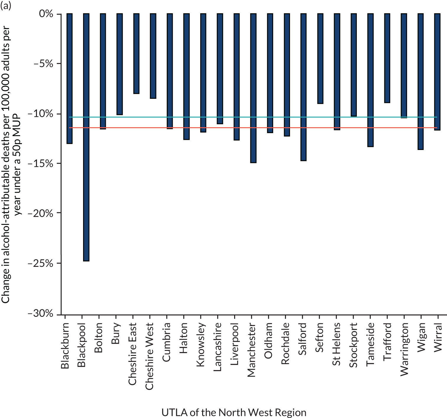
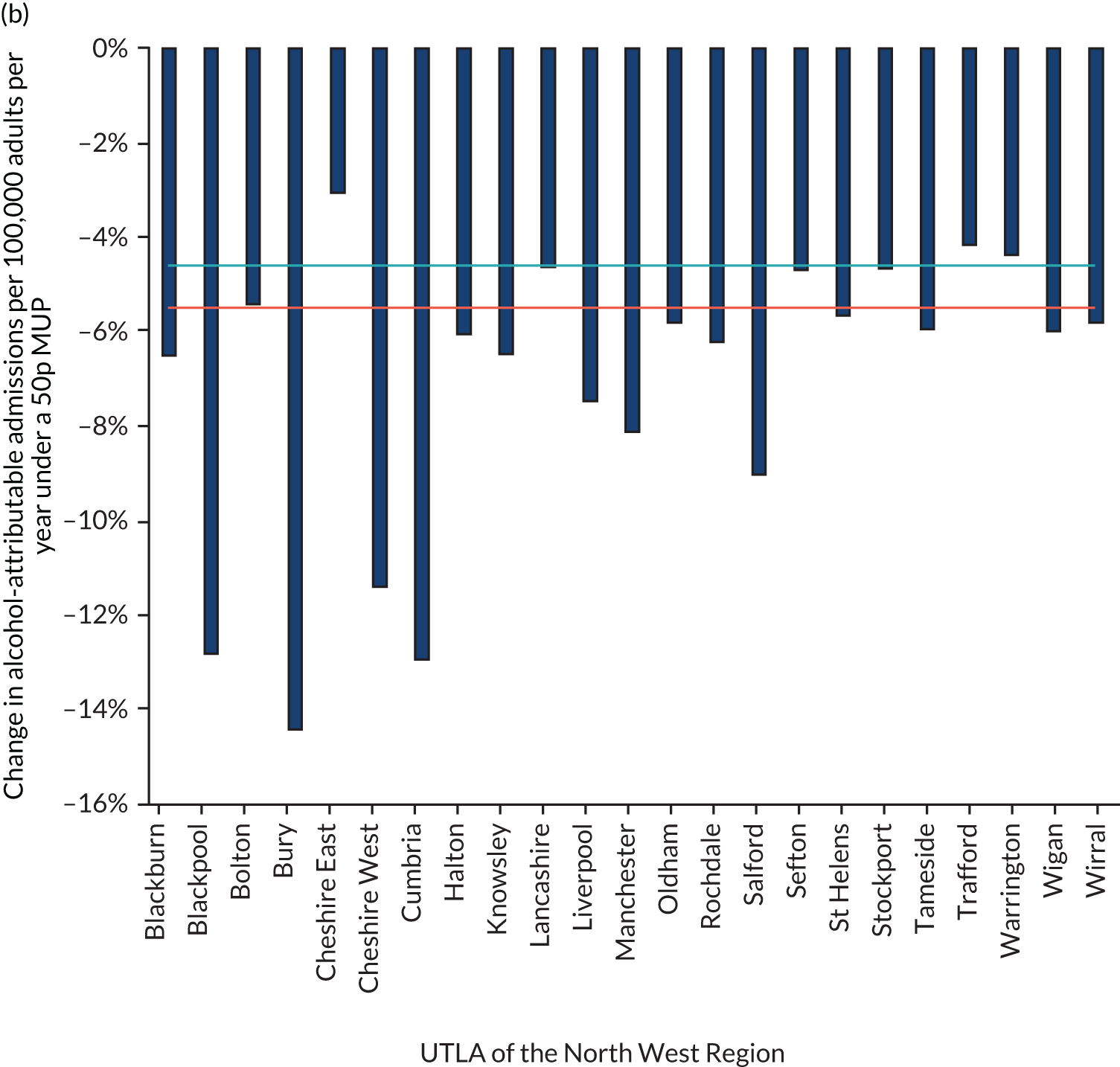
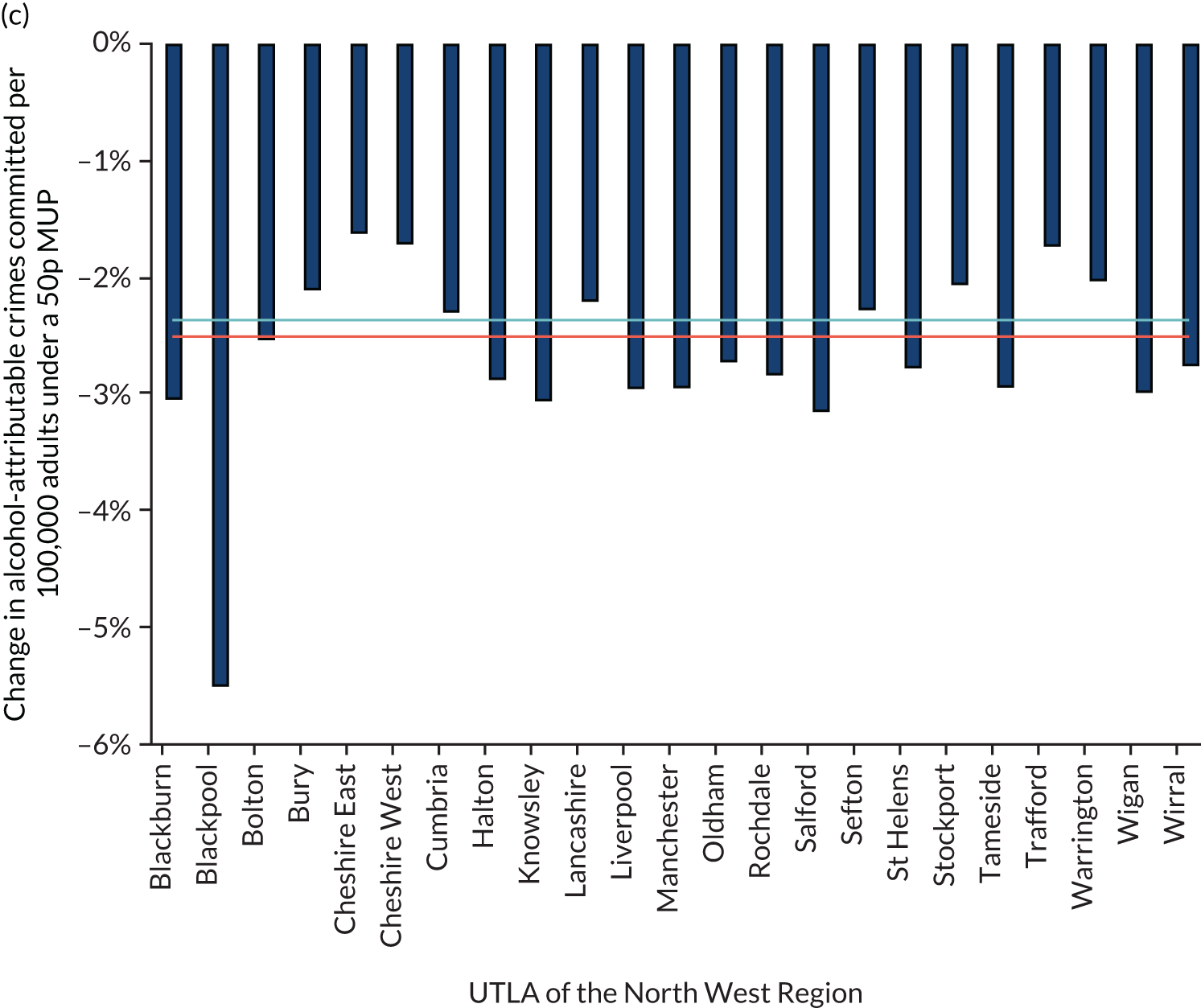
Table 11 shows the effects of the policy on consumer spending by the three drinker groups. The decreases in consumption that would drive down spending are accompanied by paying higher prices per unit, which drives up spending; for the most part, these two factors largely counterbalance each other, with relatively small increases in spending per drinker estimated to occur. For the average moderate drinker in the North West region, the change in annual spending is estimated to be just £2 per year, whereas for increasing-risk drinkers, it is £11 per year and for high-risk drinkers it is £57 per year. Overall, the effect of this is to increase revenues to the off-trade retailers (i.e. supermarkets and shops), after deducting value-added tax (VAT) and alcohol duty paid to the government, by ≈ £63M per year (an increase of 11.7%). There is a small decrease estimated by the model in after-tax revenues for the on-trade (i.e. pubs, bars, clubs and restaurants) of ≈ £4.7M per year (–0.6%, equivalent to –£7.62 per outlet per week). This small on-trade revenue change is calculated by assuming that previously seen patterns of ‘cross-price elasticities’, defined as the percentage change in consumer purchasing of on-trade products when there is a 1% rise in off-trade prices, will occur under a MUPLocal policy implementation. See Appendix 6, Table 16, for the same results for the local authorities in the North East region of England.
| UTLAs in the North West | North West | North East | National | |||||||||||||||||||||||
|---|---|---|---|---|---|---|---|---|---|---|---|---|---|---|---|---|---|---|---|---|---|---|---|---|---|---|
| Blackburn | Blackpool | Bolton | Bury | Cheshire East | Cheshire West | Cumbria | Halton | Knowsley | Lancashire | Liverpool | Manchester | Oldham | Rochdale | Salford | Sefton | St Helens | Stockport | Tameside | Trafford | Warrington | Wigan | Wirral | ||||
| Change in mean annual expenditure (£) | 5.61 | –12.86 | 7.46 | 8.92 | 9.77 | 9.88 | 8.26 | 6.39 | 6.67 | 8.30 | 5.61 | 5.90 | 6.86 | 6.84 | 3.67 | 8.38 | 6.78 | 7.70 | 5.96 | 7.75 | 8.18 | 4.45 | 6.03 | 7.11 | 2.07 | 8.89 |
| Moderate drinkers | 2.18 | –0.45 | 2.43 | 2.62 | 2.72 | 2.77 | 2.58 | 2.30 | 2.37 | 2.55 | 2.04 | 2.26 | 2.37 | 2.35 | 1.69 | 2.70 | 2.37 | 2.41 | 2.24 | 2.37 | 2.48 | 2.04 | 2.28 | 2.34 | 2.25 | 2.53 |
| Increasing-risk drinkers | 9.02 | –17.36 | 12.22 | 14.56 | 16.16 | 16.48 | 13.04 | 8.65 | 8.97 | 13.44 | 6.91 | 8.38 | 11.28 | 10.53 | 2.91 | 13.81 | 9.74 | 12.22 | 8.25 | 13.13 | 12.91 | 7.64 | 8.49 | 10.99 | 1.93 | 14.82 |
| High-risk drinkers | 50.43 | –160.20 | 63.34 | 71.26 | 72.35 | 75.85 | 63.45 | 47.93 | 52.98 | 66.66 | 50.30 | 55.30 | 58.49 | 59.09 | 31.57 | 65.29 | 51.40 | 59.87 | 47.65 | 62.39 | 63.41 | 22.56 | 43.84 | 57.23 | 0.70 | 86.95 |
| Change in revenue to retailers (£000,000) | ||||||||||||||||||||||||||
| Off-trade | 1.13 | 0.79 | 2.42 | 1.69 | 3.32 | 3.03 | 4.80 | 1.21 | 1.46 | 10.78 | 4.47 | 4.34 | 1.87 | 1.87 | 2.07 | 2.57 | 1.73 | 2.41 | 2.02 | 1.71 | 1.81 | 2.79 | 2.89 | 63.57 | 26.91 | 431.97 |
| On-trade | –0.12 | –0.38 | –0.16 | –0.08 | –0.05 | –0.06 | –0.32 | –0.12 | –0.15 | –0.59 | –0.42 | –0.36 | –0.14 | –0.17 | –0.28 | –0.14 | –0.16 | –0.15 | –0.21 | –0.06 | –0.09 | –0.36 | –0.28 | –4.68 | –4.82 | –4.52 |
We investigated alternative higher and lower thresholds for a MUP. Figure 14 shows how the estimated impact of a MUPLocal policy would differ if a threshold lower or higher than 50p were used. The results show that a 30p MUP would be estimated to have around one-tenth of the impact of a 50p MUP, and a 40p MUP would have around half of the impact of a 50p MUP, whereas increasing the threshold to 60p or 70p per unit would increase the effect by a factor of around 1.8 and 3.0, respectively.
FIGURE 14.
Effects on percentage change in alcohol-attributable deaths, hospital admissions and crimes for the range of different possible MUP thresholds in the North West and nationally. NW, North West.
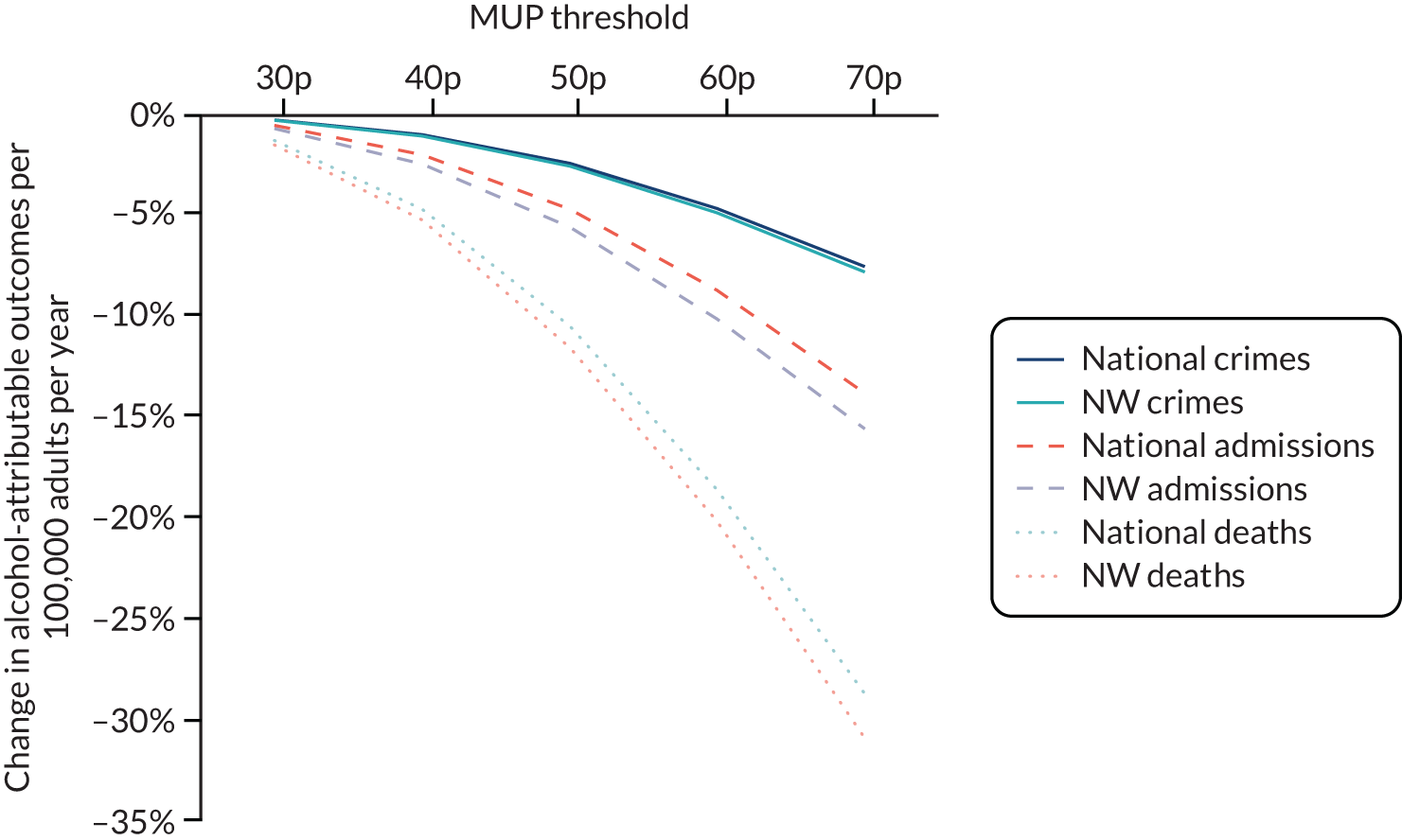
Figure 15 shows the effect of the 50p MUP policy on health inequalities, as measured using the slope index of inequality. The baseline results show that there is substantial current inequality in mortality rates between the very most and very least deprived in every local authority in the North West region (the length of the bar in Figure 15a). The impact of a 50p MUP is not only to lower the average mortality rate in each local authority (the solid dots in Figure 15b), but also to reduce the inequality between the most and least deprived. This is because the most deprived heavy drinkers reduce their consumption the most (i.e. the bar in Figure 15 would be shortened for each local authority), and because the higher end (the most derived people in the local authority) of the bar (of Figure 15) is reduced substantially more than the lower end. The reduction in inequalities for mortality is similar in relative magnitude to the reductions for the hospitalisation rate (not shown).
FIGURE 15.
Slope index of inequality (length of bars) in alcohol-attributable deaths (a) before and (b) after a 50p MUP. Circles represent the average alcohol-attributable death rate before the MUP policy and solid dots represent the rate after the policy is introduced. Dark blue shading represents changes post policy.
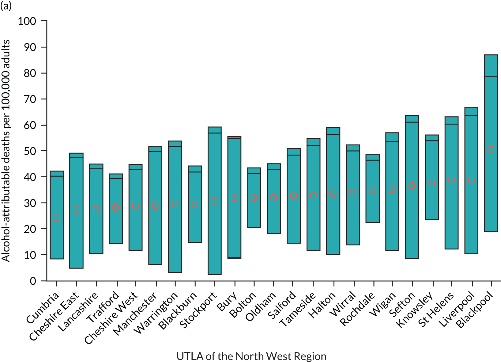
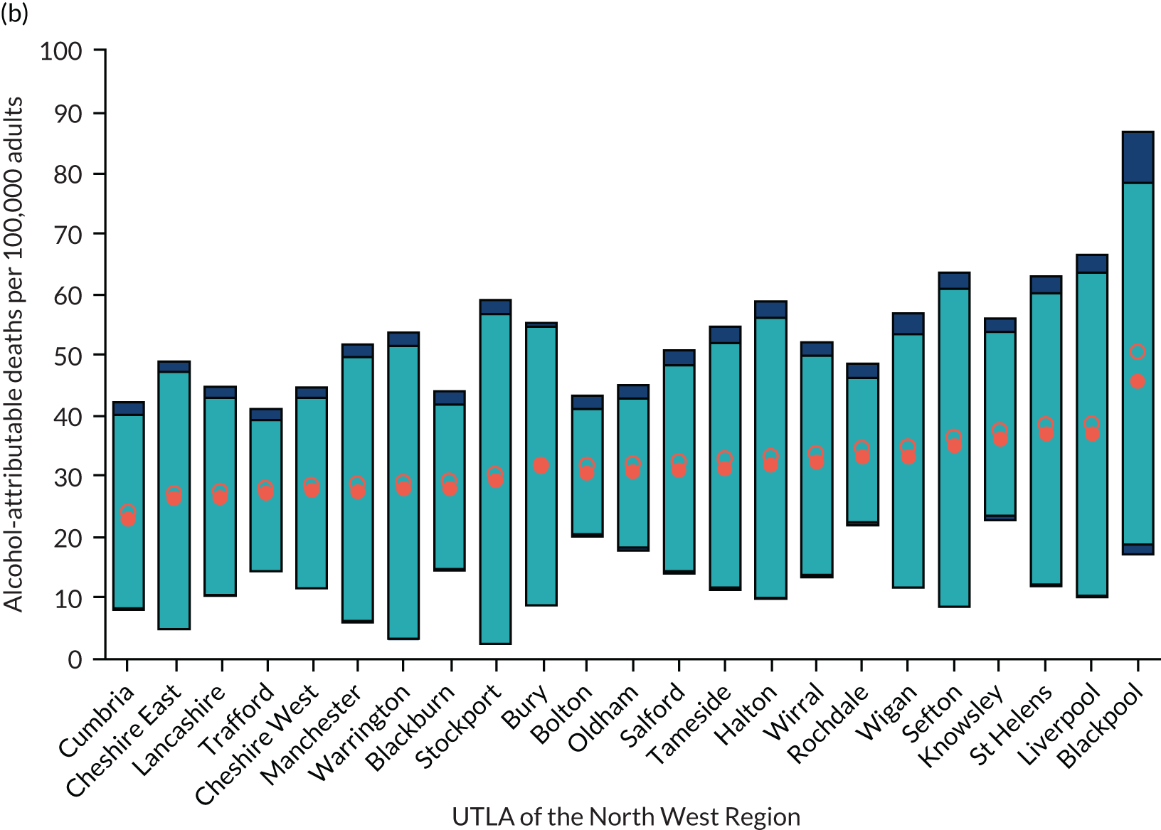
High-level two-sided summary evidence briefing results for one exemplar local authority (Sefton) and for the North West region
In this section of results, we present a high-level summary of the results for one local authority (Sefton), and a high-level summary for the results for the North West GOR as a whole. Equivalent results for the North East region and one example local authority within it (Redcar and Cleveland) are shown in Appendix 4.
This is material that has been summarised from the full set of evidence assets and discussed with stakeholders in the various meetings during the project, and is judged as being relevant to a range of audiences. It is anticipated that this material will be disseminated to key opinion leaders in the local authorities across the regions for which the analysis has been undertaken.
Two-sided evidence briefing for Sefton
The University of Sheffield logo has been reproduced with permission (University of Sheffield, 2021, personal communication).
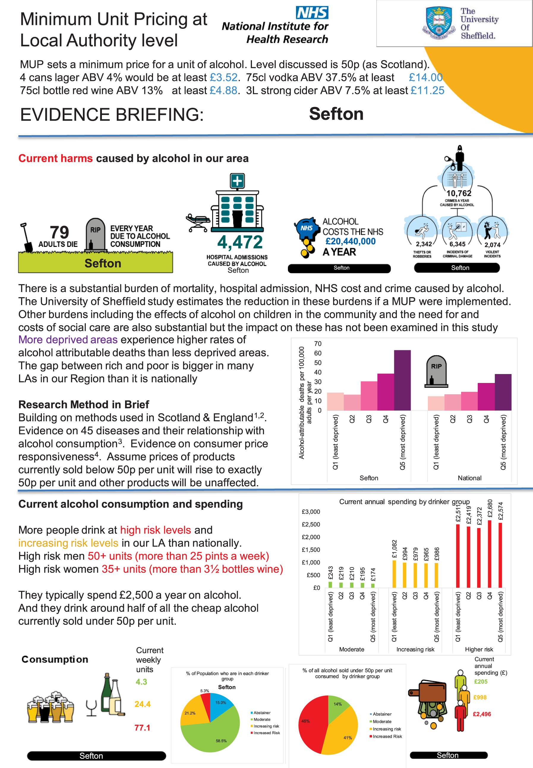
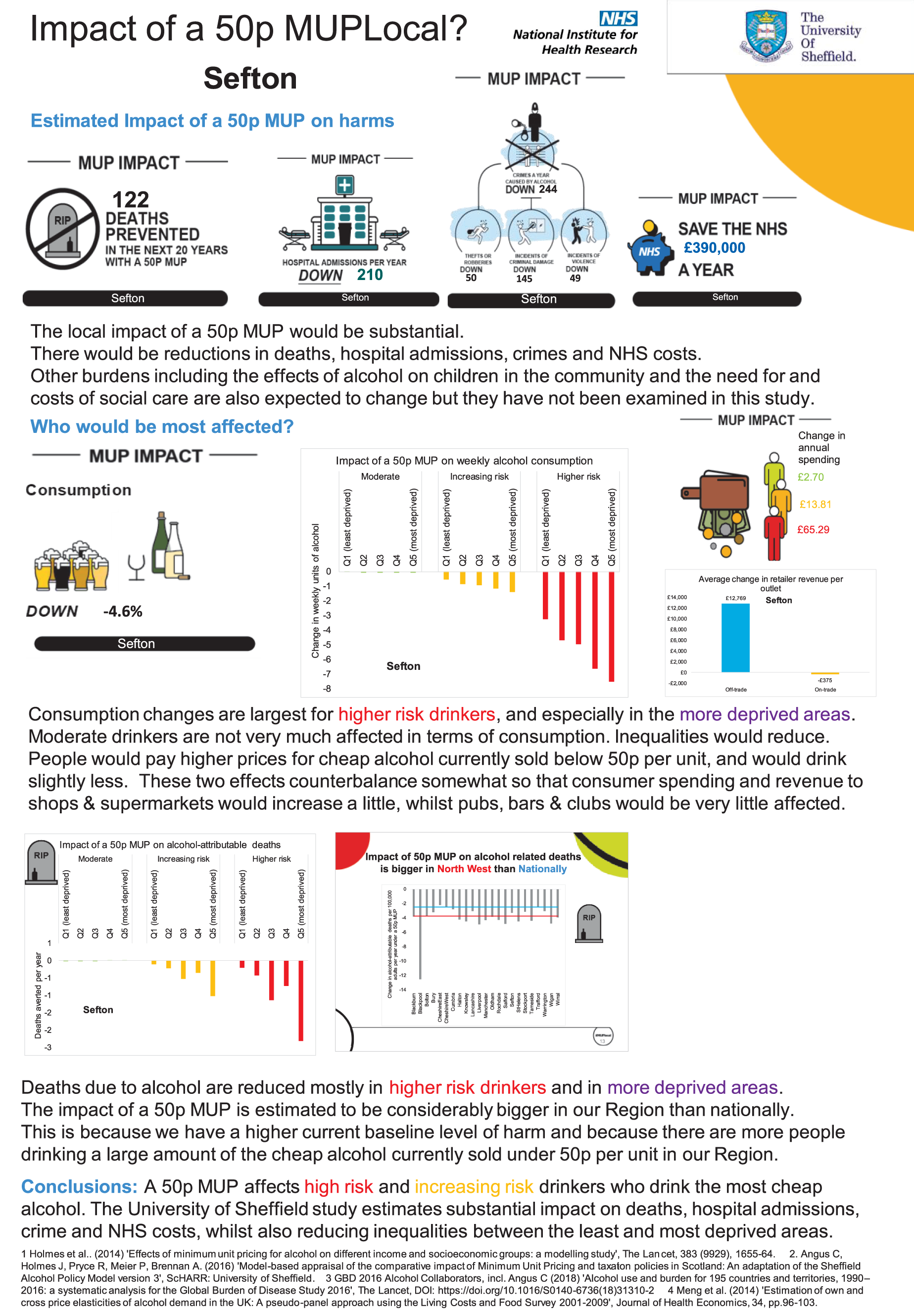
Two-sided evidence briefing for North West Government Office Region as a whole
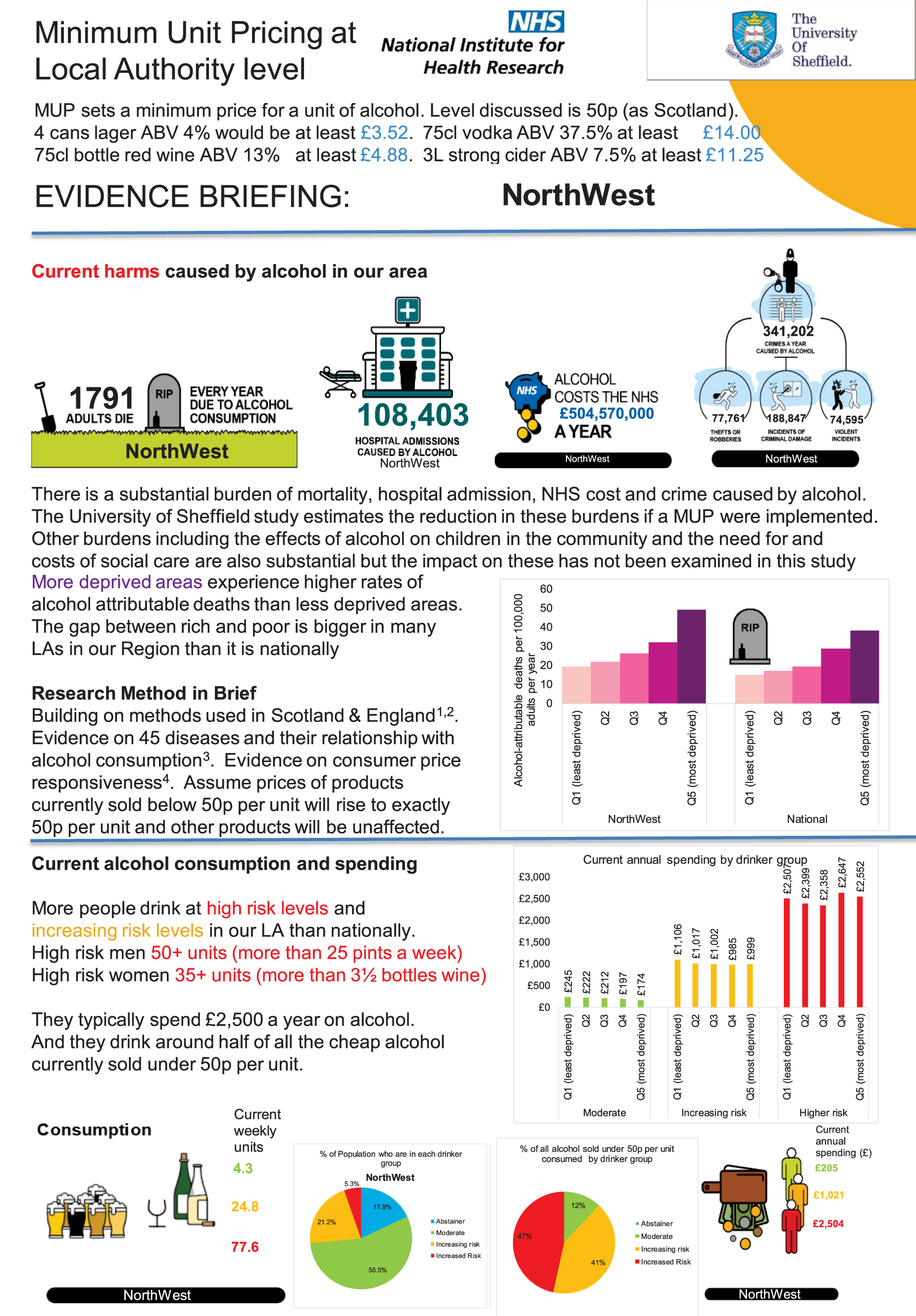

The evidence assets developed in the project: some illustrations for one exemplar local authority (Sefton)
A detailed set of evidence assets have been developed through the project with stakeholders. For each UTLA, a 65-slide PowerPoint evidence assets slide deck was developed. Draft versions of these were presented to the participants who attended the two major stakeholder meetings in the North West and North East regions on 7 November 2018 and 13 November 2018, respectively.
There are three sections to the presentation:
-
What is the scale of the problem? – This covers the harm caused by alcohol in the local authority as estimated by the SAPMLA and wider evidence.
-
Detailed patterns of consumption in the local authority at current baseline.
-
Impact of a 50p MUP on consumption and spending, impact of a 50p MUPLocal on deaths, hospitalisations, NHS costs and crimes, and implications for retailers.
It is anticipated that users of these evidence assets will mix and match slides to enable them to develop presentations for different audiences and of different durations.
The evidence assets are available for detailed review at the project website: www.sheffield.ac.uk/scharr/sections/ph/research/alpol/research/1.794701.
The evidence assets for each local authority and region modelled are available at www.sheffield.ac.uk/scharr/sections/ph/research/alpol/research/minimumunitpricinglocal/assetbank.
Ten of the key slides are presented in Figures 16–25, which provide the main analyses for the Sefton local authority. Three of the equivalent slides at national level are presented in Appendix 5, Figures 28–30.
The slide in Figure 16 summarises the big picture of the scale of the local problem in the Sefton UTLA. Every year, 79 adults die as a result of alcohol consumption and there are almost 4500 hospital admissions caused by alcohol. This costs an estimated £20M per year to the NHS in Sefton. Crime also has a substantial impact, with > 10,000 crimes per year estimated to be caused by alcohol (including accounting for those that go unreported to police): 2350 robberies, 2000 violent incidents and > 6000 incidents of criminal damage.
FIGURE 16.
Example PowerPoint slide on the scale of the problems caused by alcohol in Sefton.
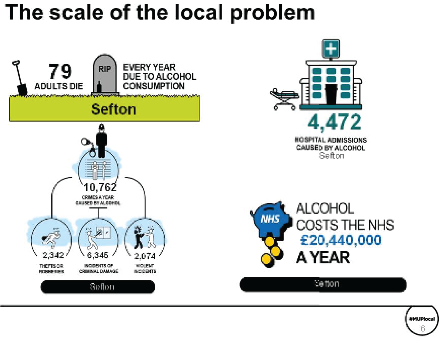
The slide in Figure 17a compares the drinking patterns for people in Sefton with the national average for England. It shows, in red, that 5.3% of people drink at high-risk levels in Sefton, which is higher than the national average of 4.5%. These high-risk drinkers are drinking ≥ 50 units per week (for males) or ≥ 35 units per week (for females). This group of people purchase 35% of all the alcohol drunk by the population of Sefton and they purchase almost half (46%) of the cheap alcohol sold at < 50p per unit. It is the amber and red groups of people that are most targeted by a MUPLocal. Only 14% of all the alcohol purchased at < 50p per unit is consumed by moderate drinkers, that is 86% of the cheap alcohol sold in Sefton is consumed by people drinking more than the Chief Medical Officer guidelines40,41 of 14 units per week.
FIGURE 17.
Example PowerPoint slide on patterns of alcohol consumption in Sefton. (a) Comparing the drinking patterns for people in Sefton with the national average for England; and (b) consumption by drinker group.
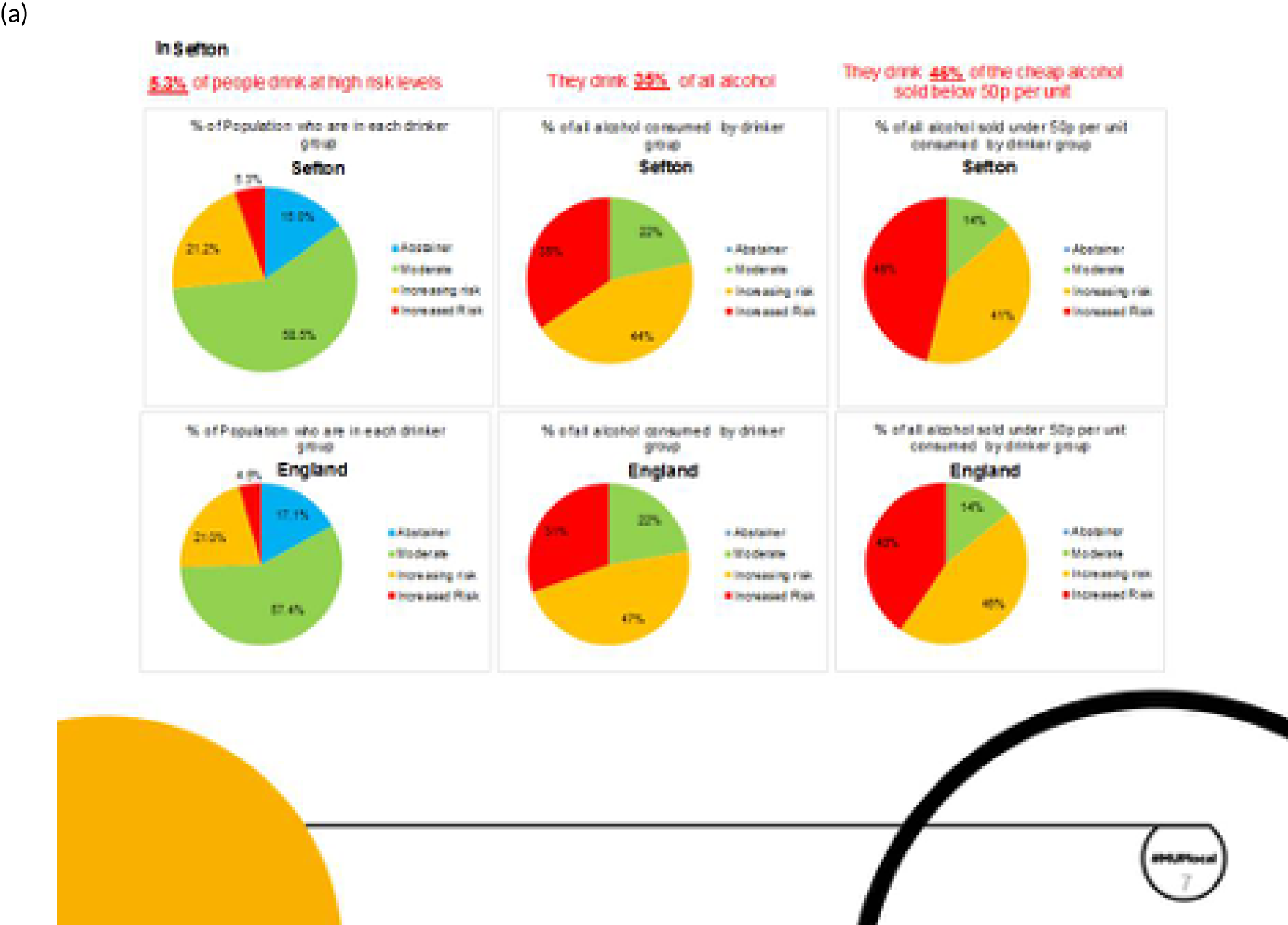
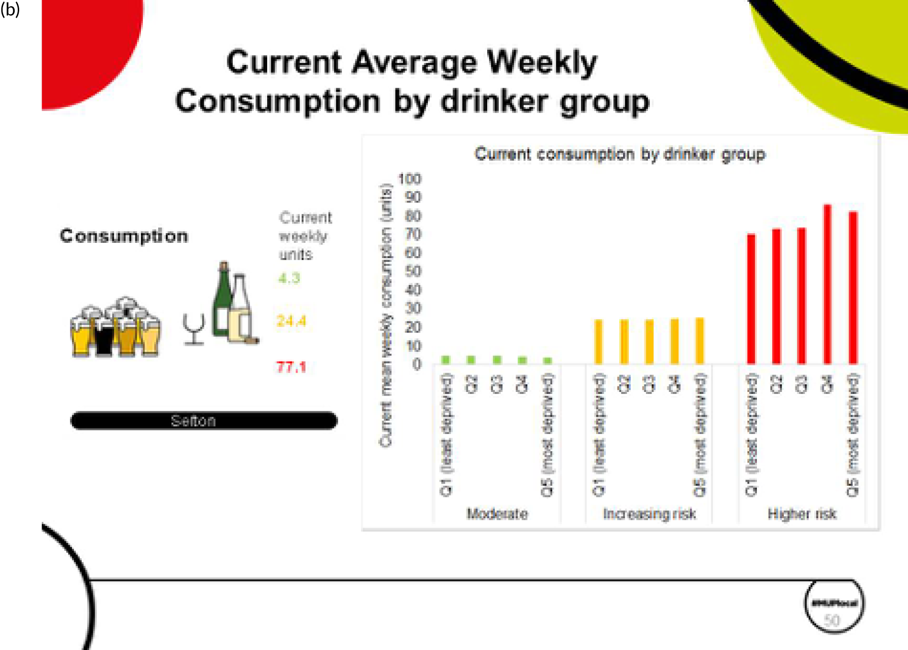
The slide in Figure 17b, for consumption by drinker group, shows that moderate drinkers, on average, drink 4.3 units per week, compared with 24.4 units per week for increasing-risk drinkers and 77.1 units for high-risk drinkers. There is no discernible difference across IMD quintile once drinker type is controlled for, apart from for the most deprived high-risk drinkers, who drink more than the less deprived high-risk drinkers.
The slide in Figure 18 shows that Sefton has a rate of alcohol-attributable hospital admissions that is higher than the national average. The Sefton rate is also somewhat higher than the North West regional average. In fact, every one of the 23 UTLAs in the North West region has a rate of alcohol-attributable hospital admissions that is higher than the national average. Some local authorities have rates that are higher than that for Sefton, for example Blackpool, Halton, Knowsley, Salford, St. Helens and Wirral.
FIGURE 18.
Example PowerPoint slide that shows that levels of alcohol-attributable admissions are higher than the national average in Sefton and in the North West region.
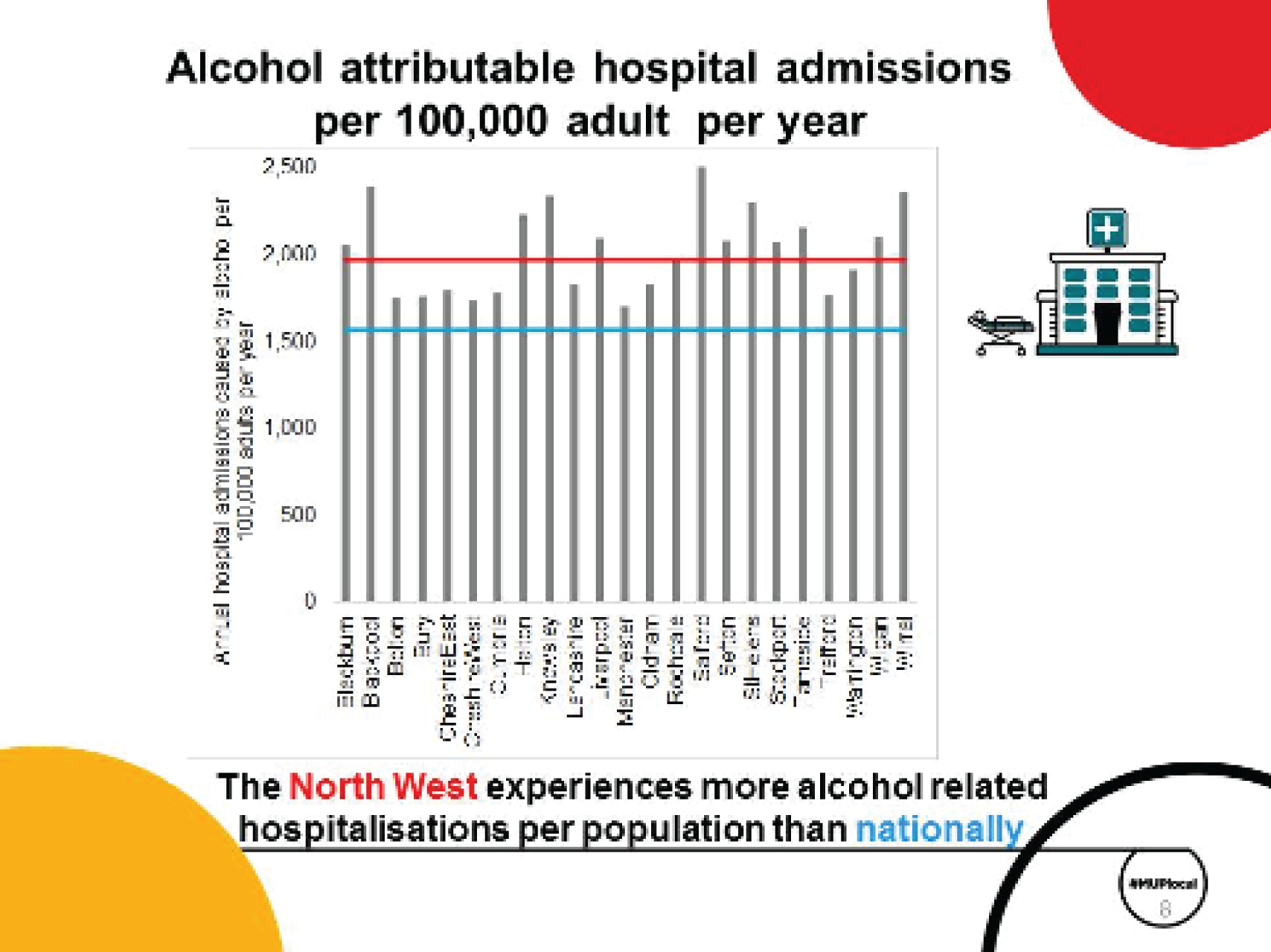
Another important factor is that people living in the most deprived areas in the local authority experience higher levels of alcohol-related harm than those living in the least deprived areas (Figure 19). This slide compares five population subgroups using the IMD, ranging from the least deprived (light pink) to the most deprived (dark purple). For Sefton, this shows that the most deprived areas have a rate of alcohol-attributable deaths that is > 60 deaths per 100,000 population, which is three times more than the level experienced for people in the least deprived or second least deprived quintile. This gap between the least deprived and most deprived areas also occurs at a national level. However, the gap between rich and poor is bigger in Sefton local authority than it is, on average, nationally.
FIGURE 19.
Example PowerPoint slide that shows that alcohol-attributable death rates are higher than the national average in Sefton, especially among those who live in the most deprived areas.
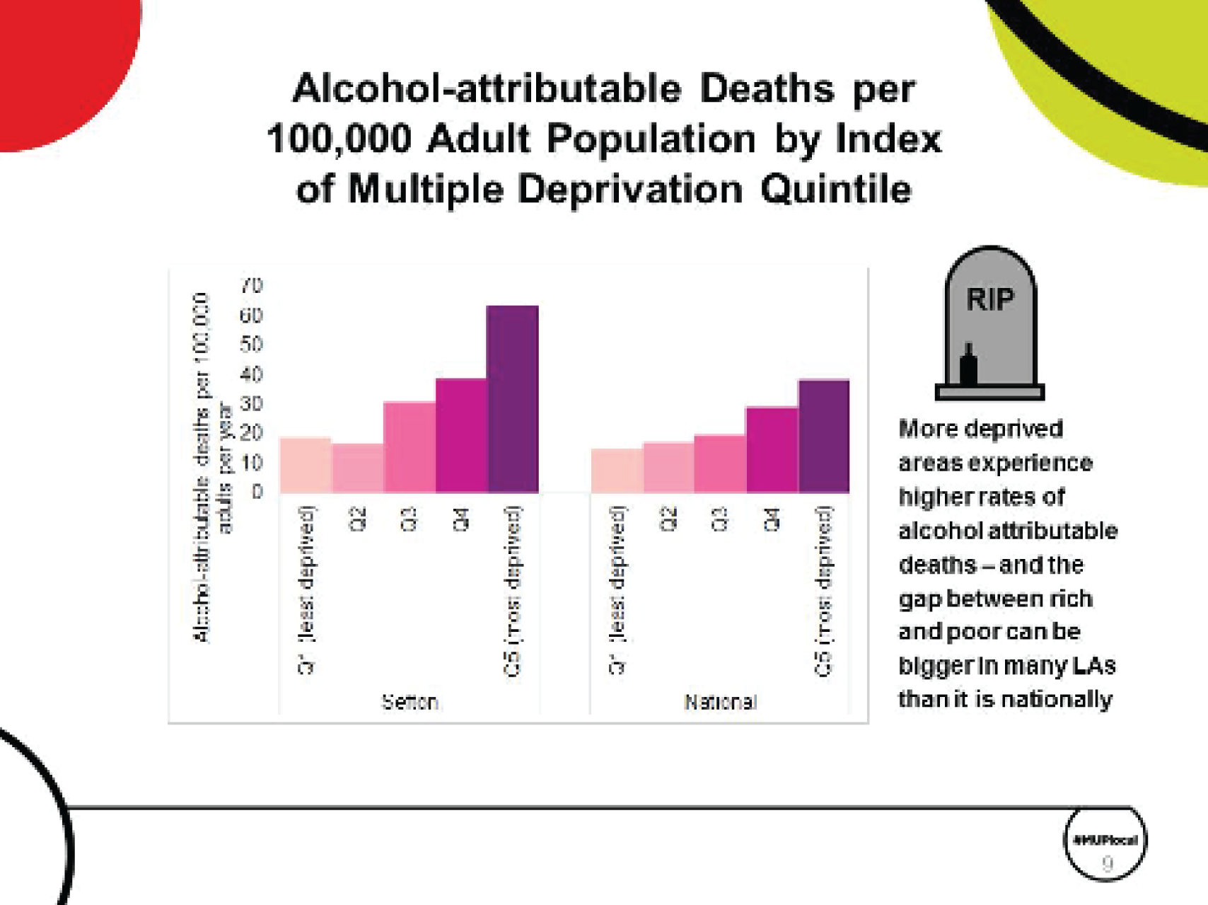
Figure 20 summarises the impact of a 50p MUP in Sefton. It is estimated that, over the next 20 years, the policy would prevent 122 deaths due to alcohol.
FIGURE 20.
Example PowerPoint slide showing the impact of a 50p MUPLocal in Sefton on alcohol-related harm.
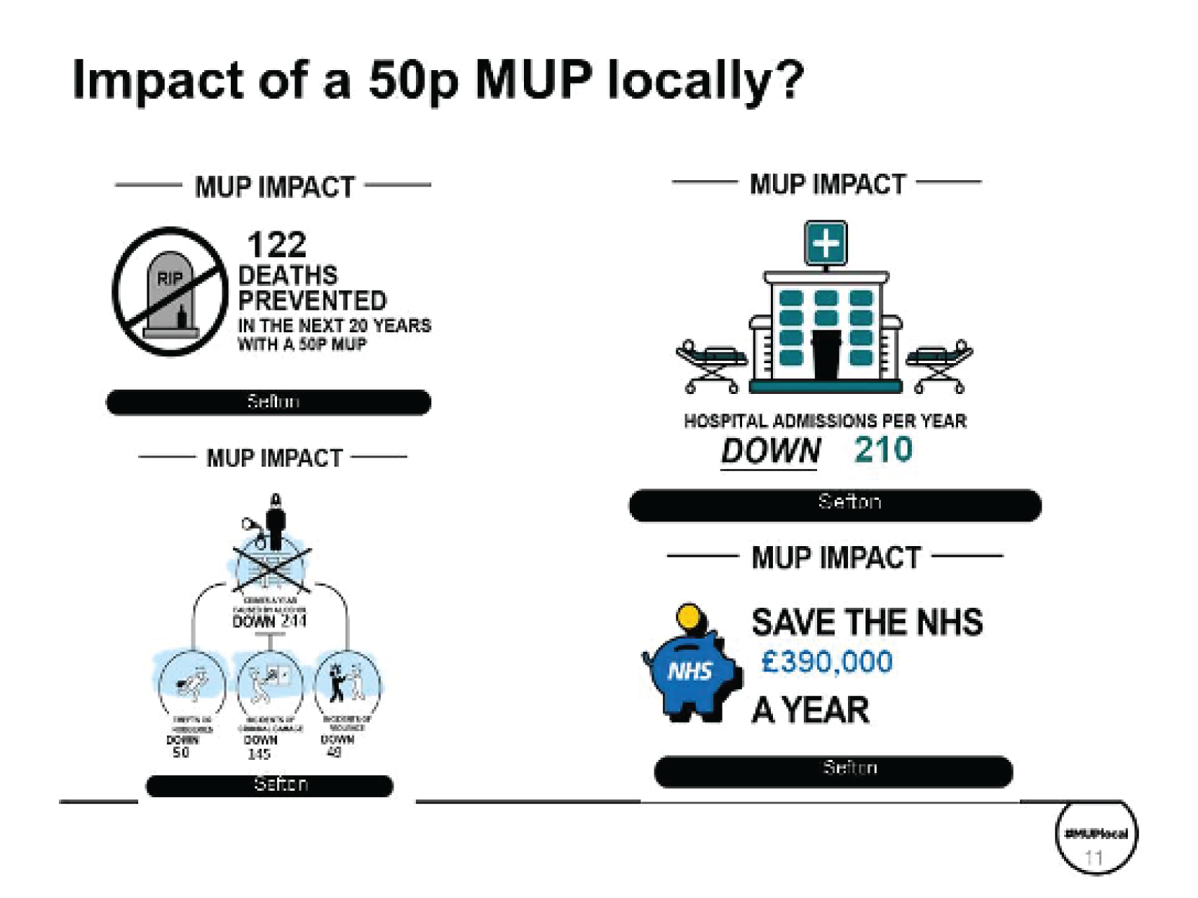
Hospital admissions due to alcohol would be down annually by 210 admissions. This would save the NHS around £390,000 per year.
In terms of crime, we estimate a reduction in the number of crimes caused by alcohol of just under 250 per annum: 55 fewer robberies, ≈ 50 fewer incidents of violence and ≈ 145 fewer incidents of criminal damage.
These impacts on harm come about because of reductions in consumption (Figure 21). On average, total consumption of alcohol is estimated to decrease by ≈ 4.6% in Sefton. The reductions are occurring mostly for people in the high-risk (red) and increasing-risk (amber) groups in the population. The graph shows that moderate drinkers reduce consumption by only very tiny amounts. In contrast, high-risk drinkers reduce their consumption by between 3 and 7 units per week, with those in the most deprived areas reducing their consumption the most.
FIGURE 21.
Example PowerPoint slide showing changes in consumption for moderate, increasing-risk and high-risk drinkers, split by IMD quintile.
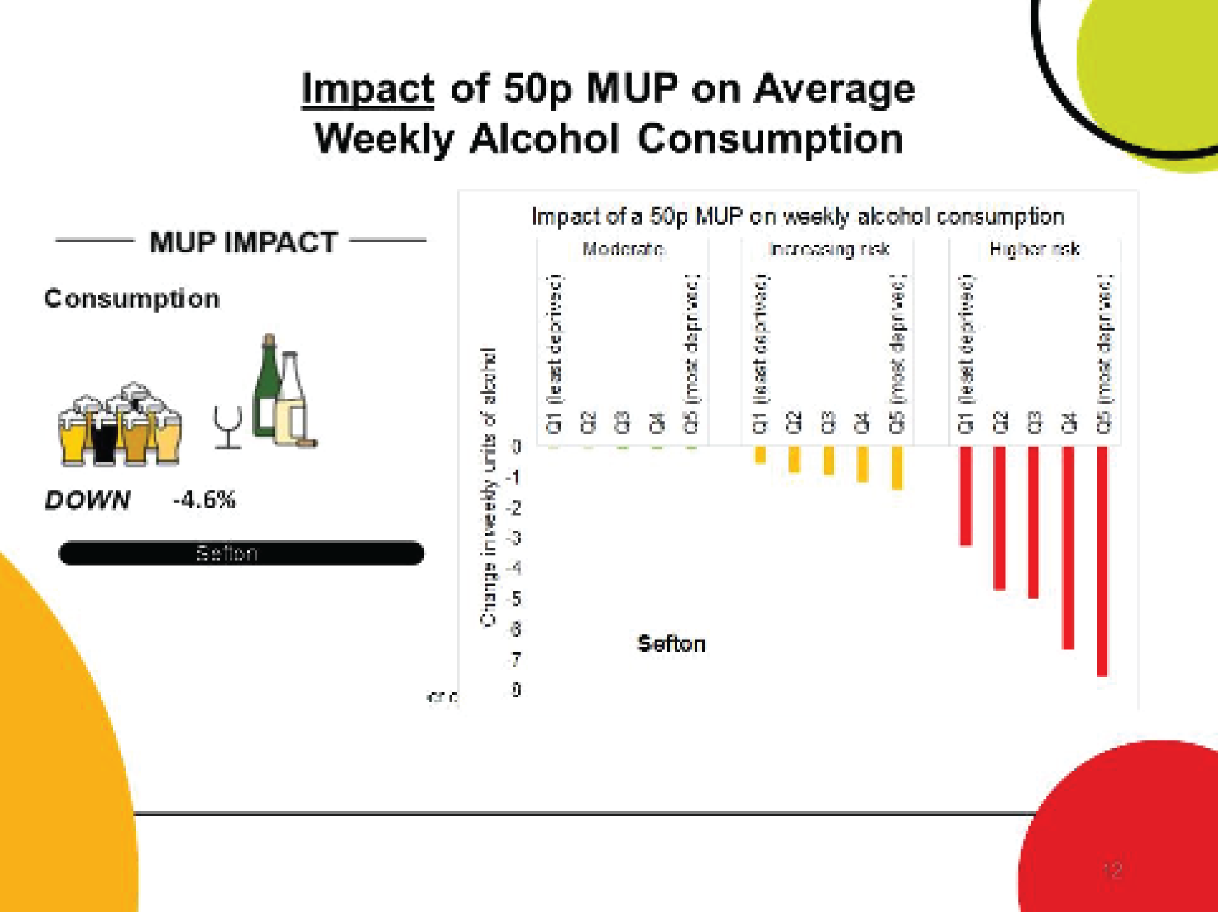
Figure 22 shows that the impact of a 50p MUP in terms of reduction in alcohol-attributable deaths per 100,000 population for Sefton is larger than it is for England as a whole. Indeed, all but one of the local authorities in the North West region are estimated to have a greater reduction in deaths than the national average. Blackpool is a particular outlier, with a large baseline number of deaths attributable to alcohol and a large proportion of people who are in the high-risk group who drink a lot of alcohol that costs < 50p per unit. Blackpool’s estimated reduction in alcohol-related deaths is the largest of any other tier local authority examined in this study. Figure 22b shows that the impact on alcohol-related deaths is bigger among people who are higher-risk drinkers and in deprived areas.
FIGURE 22.
Estimated reductions in alcohol-attributable deaths due to a 50p MUP (a) comparatively across UTLAs in the North West; and (b) compared by drinker group and deprivation.
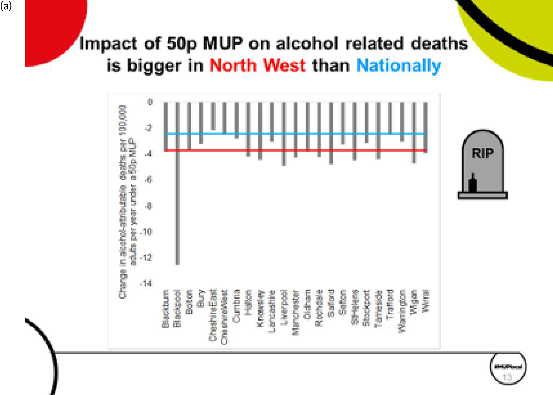
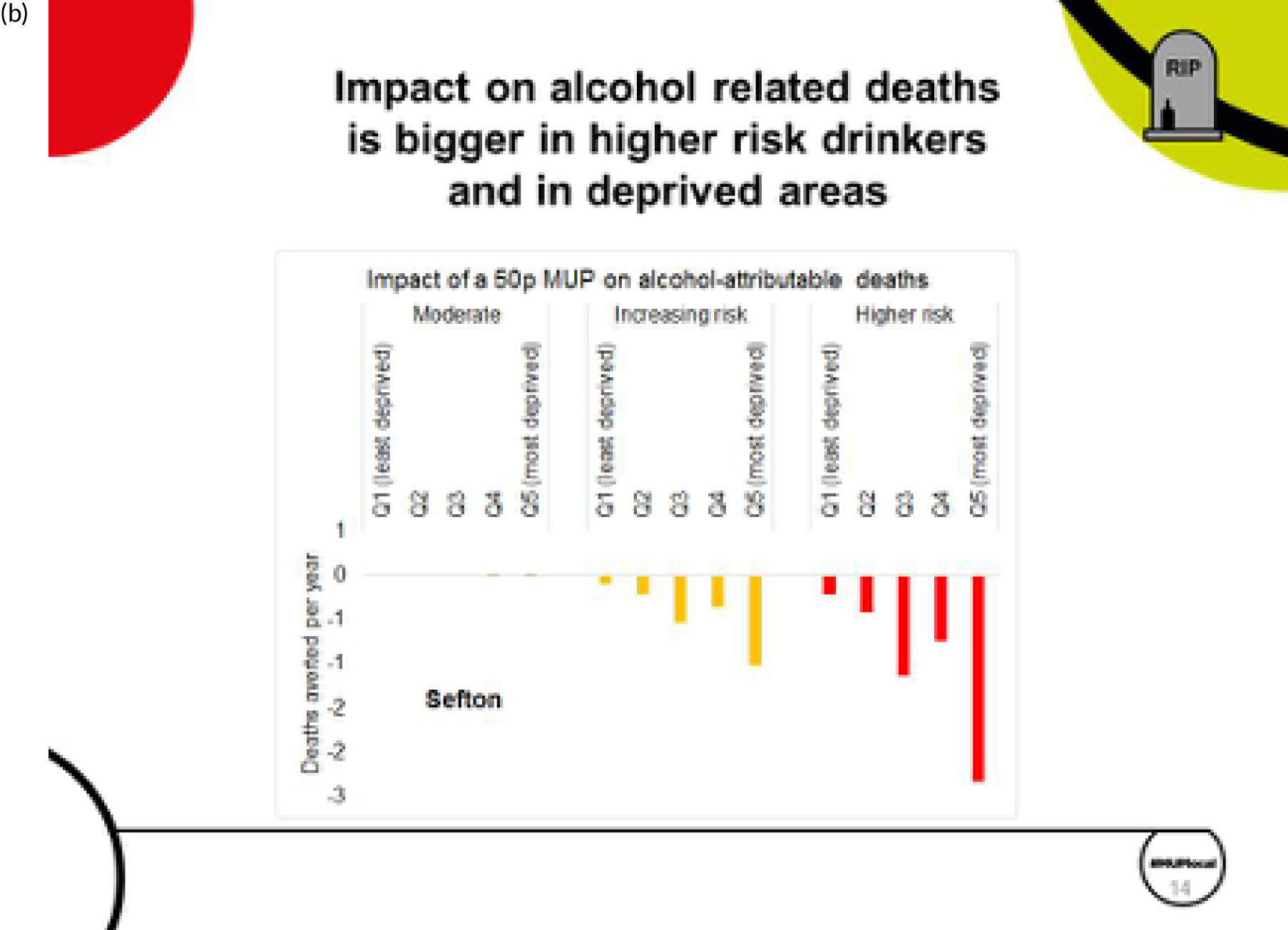
Baseline spending patterns in Sefton (Figure 23) show that the average moderate drinker spends £205 per year on alcohol, compared with £998 for increasing-risk drinkers and £2496 for higher-risk drinkers. Among the moderate and increasing-risk drinkers, the least deprived spend slightly more per year. However, this difference is not seen among the higher-risk drinkers.
FIGURE 23.
Estimated spending by consumers. (a) Current spending; and (b) change in spending due to implementation of a 50p MUP.
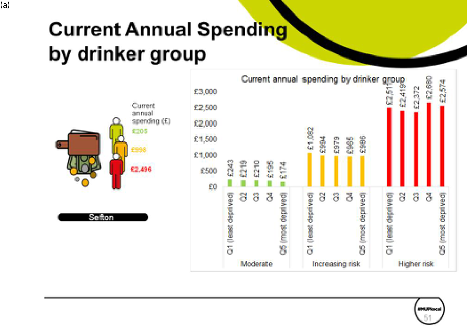
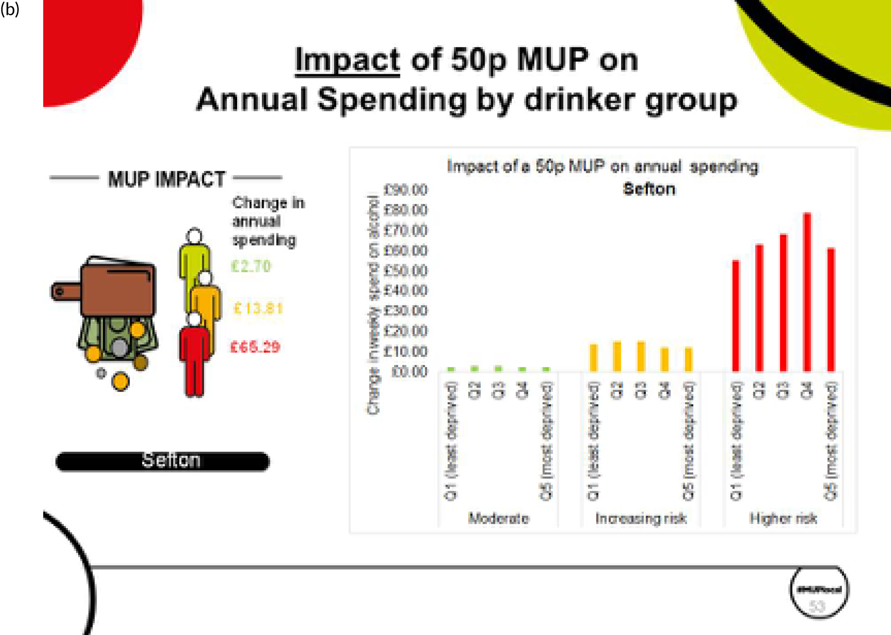
We estimate that a 50p MUP in Sefton would result in an increase in expenditure for all drinker types, on average. Moderate drinkers would increase expenditure on alcohol by £2.70 per year, whereas higher-risk drinkers would increase spending by £65.29 per year. There is no large difference by deprivation quintile among moderate and increasing-risk drinkers, but there are such differences among higher-risk drinkers.
When prices rise, and consumption falls, there will be an effect on spending and, of course, on retailers’ revenues. For most of the analyses we have undertaken, the decrease in consumption is smaller than the increase in prices, meaning that the net effect is that people drink a little less and spend a little more. Figure 24 shows that the effects of minimum pricing are seen almost entirely in the off-trade (shops and supermarkets). This is because very little alcohol sold in on-trade (pubs, bars, clubs, etc.) is sold at < 50p per unit. Therefore, the impact of a MUP is mostly seen as an increase in retailer revenue in supermarkets and shops. For Sefton, we estimate an increase in retailer revenue in the off-trade of ≈ £2.6M per annum. For pubs, bars and clubs in Sefton, we estimate a possible tiny reduction in retailer revenue. The reason there is an estimated reduction in on-trade revenues is that we utilise previously published national evidence on ‘cross-price elasticities’. For example, Table 5 showed that a 1% increase in price of off trade cider, would be estimated to produce a reduction in the purchasing of on-trade beer of –0.053%. Table 5 also showed that a 1% increase in price of off trade cider, would be estimated to produce an increase in the purchasing of on-trade cider + 0.093%. The model aggregates all of these small and different direction cross-price effects for the different beverage categories and produces an overall estimate of the change in on-trade consumption if a MUP were implemented. It is important to note that all of these cross-price elasticity effects are quite small in our model, and also somewhat uncertain, from the historical evidence.
FIGURE 24.
Estimated impact on alcohol retailers’ sales. (a) Per annum in Sefton; and (b) per annum per outlet in Sefton.
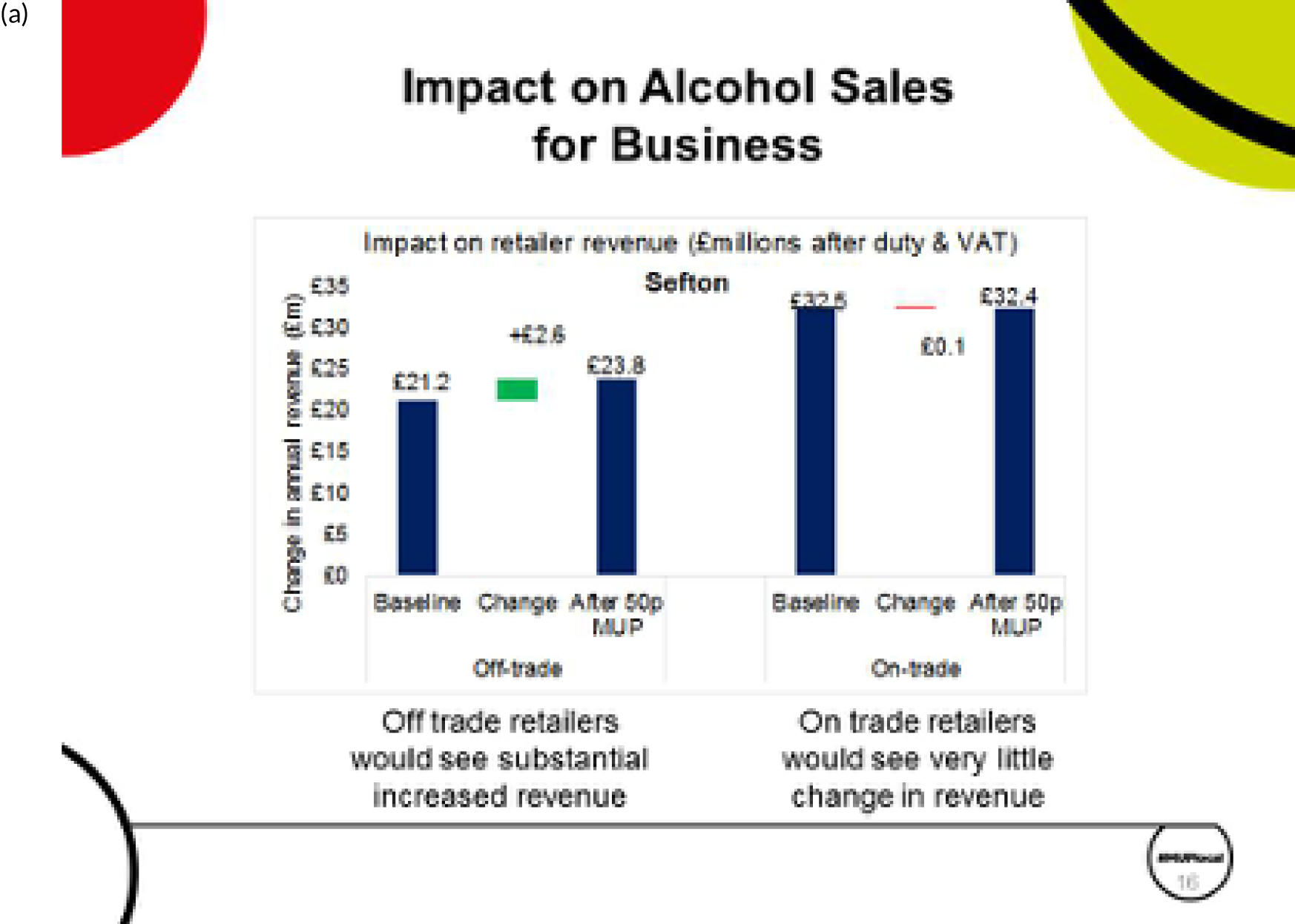
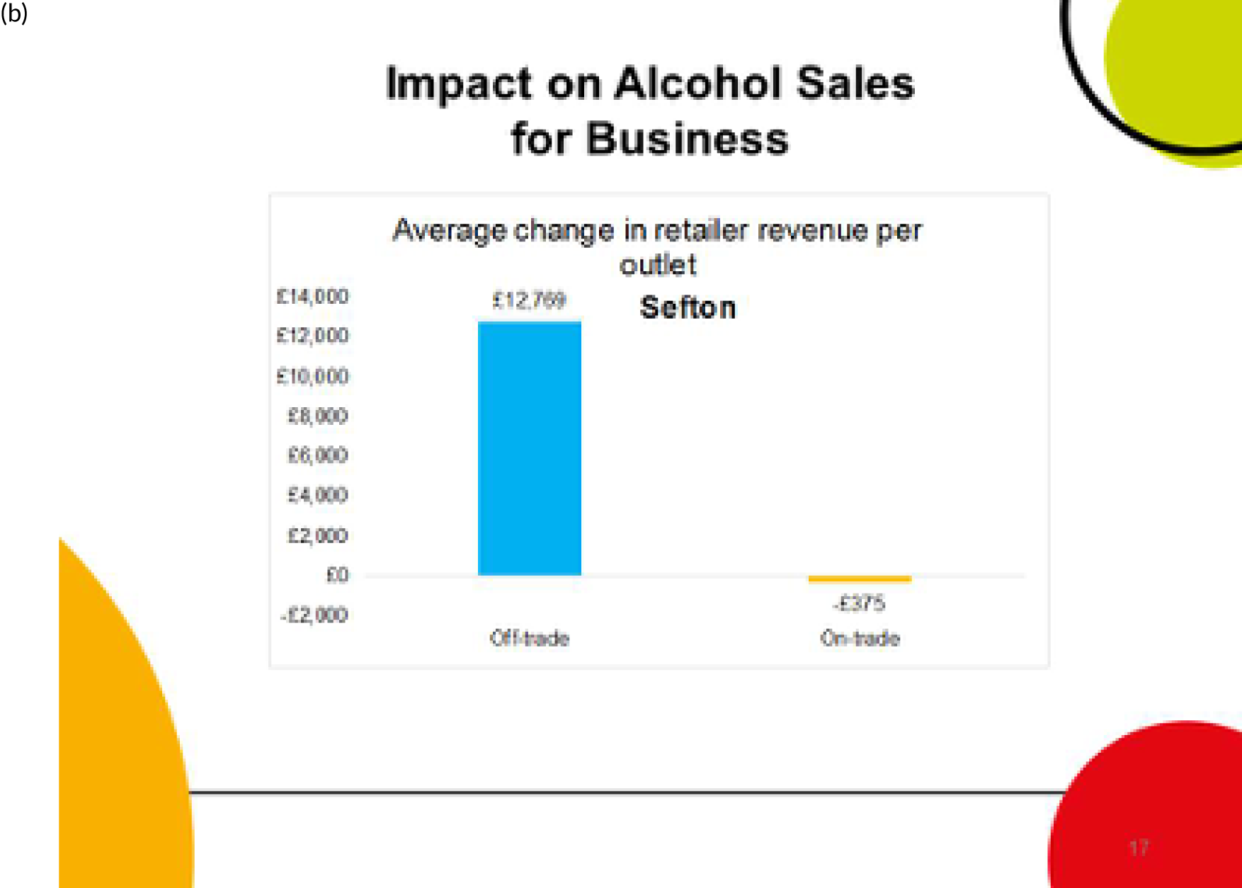
A minimum unit pricing policy is not a tax policy, so the additional money does not go directly to government; it goes to the retailers selling the products. There are some impacts on tax revenues because less alcohol is sold, which reduces alcohol duty receipts for the government, but it is sold at a higher price and with a higher sales value, thereby increasing VAT receipts. These two effects counterbalance each other somewhat, so the effects on tax receipts are not large.
Five different scenarios were examined for the threshold of a MUP for alcohol: 30p, 40p, 50p, 60p and 70p (Figure 25). On each of the measures of impact, reductions in deaths, hospital admissions, NHS costs and crimes, a 50p MUP is estimated to be around 10 times more effective than a 30p MUP threshold, and around two times more effective than a 40p MUP threshold. This is for two reasons: first, a lower threshold means that fewer products are affected by the policy, and, second, when the prices are increased, they increase by a smaller amount, for example up to 30p per unit, rather than bigger increases to 50p per unit.
FIGURE 25.
Example PowerPoint slide showing the relative impact of different MUP thresholds on measures of harm reduction in Sefton.
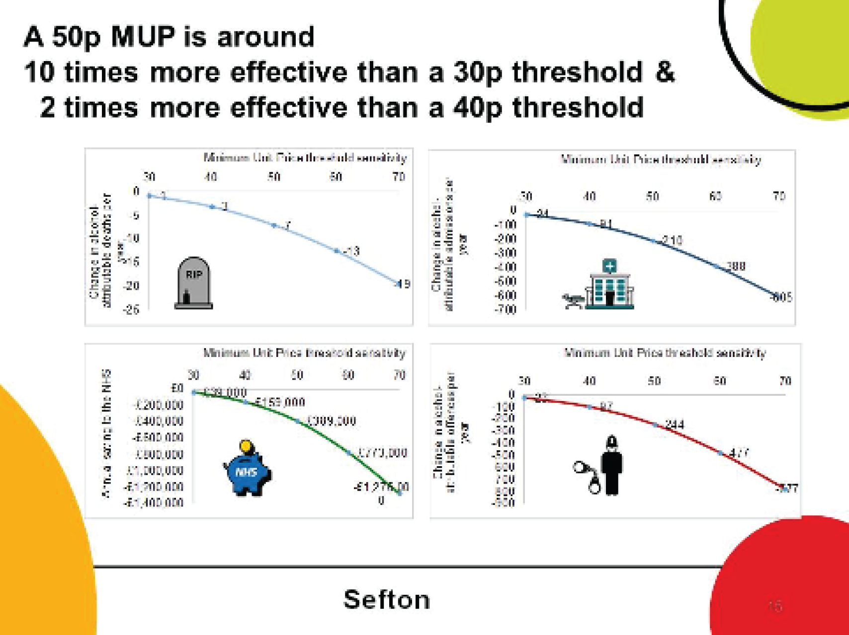
Chapter 4 Discussion
Summary of key findings
This is the first study to examine the effectiveness of a MUP for alcohol at UTLA and regional levels in the UK, to our knowledge. It utilises newly available market research data on regional differences in preferences for and price distributions of 10 categories of alcohol, synthesised with local data on alcohol-related mortality and hospitalisations for 45 conditions and alcohol-related crime data for 14 categories of offence. The results from the SAPMLA show that a 50p MUP would be an effective policy in reducing alcohol-related deaths, hospitalisations and crimes for every UTLA and GOR in England. There would be a greater impact in places with a greater prevalence of heavy drinking, higher current levels of cheap alcohol purchases and higher current levels of harm. This means that a 50p MUP would have greater effects in the North East and North West regions than in the South East and London regions. The majority of the impact occurs in those 4–7% of people in the population who drink at ‘high-risk’ levels, because these are the people who drink substantial amounts of very cheap alcohol, spending, on average, ≈ £2500 per year (broadly the same spending whether they are from the least deprived or most deprived neighbourhoods in the country). In addition, these people suffer the most current harm. A further important impact of MUPLocal as a policy is that it reduces health inequalities, because there is a higher mortality rate for those in the most deprived neighbourhoods.
Strengths and limitations
The analysis undertaken in this study builds on and adapts previous national-level work. 8–12 A key limitation (and strength) is that this demands synthesis of evidence from multiple sources, as there is no single longitudinal individual-level data set measuring alcohol consumption; prices paid; or incidences of diseases, mortality or crime. The price elasticities used are based on a detailed analysis of 9 years of the LCFS,48 as in previous national-level analyses and as used for the Scotland modelling. In previous studies,9,11,46 we examined the sensitivity of results to using alternative price elasticities and showed that effects could be somewhat higher or lower than our base-case estimates, but that patterns of impact (e.g. comparing moderate, increasing-risk and high-risk drinker subgroups, or comparing 30p, 40p, 50p, 60p and 70p thresholds) remain broadly the same. The MUPLocal results here will be subject to the same levels of relative change in results if different elasticities are used. Our analysis assumes that the population will not have access to alcohol below the MUP threshold, with no ‘cross-border’ purchasing of cheaper alcohol outside the geography where a MUPLocal is set. If MUPLocal were implemented in just one local authority, then such cross-border purchasing would be likely to dilute the effects estimated here to a greater extent than if a large group of UTLAs, a full region or a set of regions implemented MUPLocal together. Our analysis is conservative in that it models changes to the prices only of products currently below the modelled MUP threshold, and we have not made any assumptions about how suppliers or retailers might adjust prices upwards for products currently higher than the threshold. In general, when there are data limitations, the SAPM base case uses conservative assumptions, and when we previously compared results for the Canadian adaptation of the SAPM with the observed impact in Canada, we found that the model underestimated the effects of changes in MUP. 72–74 Deep discussion of the strengths and limitations of the SAPM has occurred over the preceding 10 years through scientific peer review on major research reports and in leading academic journals. There have also been some critiques of the SAPM produced by consultants commissioned by the alcohol industry75 (for details of how this was used by the alcohol industry in lobbying see76) and a free market-oriented think tank;77 the detailed rebuttal to these has been part of the evidence reviewed by the Scottish, European and, most recently, the UK Supreme Court. 78
Implications for local policy and decision-makers management (and) practice
The implications for local policy and decision-makers are, in one sense, straightforward. The model estimates suggest that the policy would be effective in substantially reducing alcohol-related harm, especially among those drinking at high-risk levels, and also in reducing inequalities between areas of least and most deprivation. This level of evidence synthesis and modelling is similar to that undertaken for Scotland, which was heavily scrutinised through the policy development processes and the legal cases. 13 The implication is that UTLAs might well want to use the evidence developed here to move forward with plans to implement a MUPLocal policy. The next step for localities and groups of localities would be to decide how to take these findings forward. One option that some UTLAs have considered is an application to the UK Home Secretary to implement a MUPLocal via a law called the Sustainable Communities Act. 14 This would require (1) evidence on the likely impact of the policy on the health and well-being of the local population and (2) there to have been a public consultation exercise. The evidence provided in this study delivers the first and could provide the basis for the latter.
The implementation of a national MUP would be a decision for the UK government, which currently takes the position that it is reviewing and considering the evidence on an ongoing basis, so the evidence presented here will be included in those processes.
There are wider implications in terms of the potential application of some of the methods we have developed here to other related topics. The fact that it has proved feasible to generate synthetic estimates of alcohol consumption and purchasing at local level could be extended to other ‘unhealthy commodities’. For example, it would be possible to utilise some of the methods described to estimate local area consumption and purchasing of tobacco products, using the HSE and the LCFS. These data sources could also potentially be used to examine unhealthy food purchasing patterns. An integrated analysis of food, alcohol and tobacco consumption and purchasing could also be possible. Academics, research funders and PHE, together with local authorities, could potentially develop these approaches further. This is not straightforward, and, reflecting on our experience, we perceive some of the key barriers to and facilitators of this to be as follows. First, there needs to be a process of examining the data in the HSE and the LCFS to understand their patterns and vagaries. For example, the exact definitions of alcohol products are different between the two data sets, and there can be issues with exactly what units are used to measure the levels of consumption and purchasing. Second, to do the regressions to estimate local re-weighted surveys, a combination of individual-level factors and local area factors should be used. There will be myriad options for the local-level factors that could be associated with (and, therefore, predictive of) local consumption of, for example, tobacco or high-fat foods. The development of appropriate regressions should be informed by a combination of theoretical models and empirical experimentation, and the science of these associations will develop over time as research groups and local authorities contribute to the processes and development of the evidence. Third, the statistical code to undertake the work has been developed in a combination of Stata® (StataCorp LP, College Station, TX, USA) and R (The R Foundation for Statistical Computing, Vienna, Austria), but requires access to confidential data sets through the UK secure data service; therefore, there is a series of information governance steps to go through in terms of access to information, protocols for analysis, extraction of results and information-sharing.
Further research and possible extensions to the analysis
In terms of further research, two key components of the harm caused by alcohol at a local level remain unexamined in this study. The first of these is the impact of a MUPLocal on social care harms and costs, in particular the risks and harms that children experience as a result of parents’ and carers’ alcohol consumption. The second is the workplace outcomes and subsequent economic consequences across the full range of sectors and industries caused by alcohol use of their own staff or those of the organisations on which they rely or with which they trade. Both of these topics were heavily discussed during our project stakeholder engagement processes, and we would strongly recommend further research to develop a quantified understanding of the additional impact of these two factors. In addition to this, evidence from Scotland on the extent of cross-border purchasing, when it emerges, could potentially be included in further analyses of any specific set of UTLAs planning to implement a MUPLocal collectively.
In terms of generalisability of findings, it is clear that the results for different UTLAs vary substantially and one cannot easily make an estimate for the English local authorities in geographies that we have not explicitly modelled. It is clear, however, that there are several consistent patterns in the estimates – moderate drinkers would be much less affected by the MUPLocal policy than high-risk drinkers, and high-risk drinkers, especially those in deprived areas, tend to experience the biggest impact and health gain. This is reflected in comparisons across local authorities, with those local authorities that have more people drinking very cheap alcohol, and those with higher deprivation, tending to see larger estimated policy impact than other local authorities where people tend to spend more on their alcohol purchases and where there is a smaller population in deprived areas. The SAPM approach has been undertaken in several countries already, with further projects under way in Australia. If data similar to those used in this study were available at regional or local level in other countries, then it would be fairly straightforward for those countries to develop a SAPMLA version of the modelling approach.
Conclusions
In conclusion, this study has enabled the generation of estimates of impact of a proposed MUPLocal policy.
These estimates suggest that the policy would be more effective in the North West and North East of England than it would be on a national basis for England. This is because local authorities in these regions tend to have a higher proportion of their population drinking at high-risk levels; tend to have higher baseline levels of harm, including alcohol-attributable mortality, hospitalisation and crime, than the national average; and because they tend to have a higher proportion of their population who drink more of the very cheap alcohol that is sold at < 50p per unit. Our study synthesises the evidence on consumption, purchasing and harms to estimate impact, which suggests that there could be substantial reductions in mortality, hospitalisation rates, NHS costs and crime rates. The estimates also suggest that there could be reductions in health inequalities because it is the high-risk drinkers in the more deprived areas who experience the most harm and would benefit most from the increase in the price of this cheap alcohol.
There are limitations and caveats in the analysis, and it will be important to consider evidence from the implementation of a MUP in Scotland as it emerges, including any evidence on the extent of ‘cross-border purchasing’.
Our analysis excludes estimating the impact on reductions in the need for social services support and costs for children, and excludes the effects on work productivity and employer costs at local authority level if there were to be lower alcohol consumption and fewer resulting illnesses, hospitalisations and crimes occurring. These are priorities for further research.
In terms of implementation, these results will enable local decision-makers to consider options on how to collaborate and take forward any plans or proposals for a MUPLocal. They provide a more developed evidence base for the likely impact of a MUPLocal and a mechanism for undertaking wider public consultation if local authorities decide to move forward with a MUPLocal.
Acknowledgements
We are grateful to Naomi Gibbs, Jenny Doole and Heather Mottishaw in our own team for support with the stakeholder events. Thanks to Sacha Wyke of PHE for provision of data.
Thank you to Ali Wheeler for support with stakeholder events, Jude Hackett, Gary Wootten and Jon Dickson at Hitch Marketing for support with Infographics; Colin Shevills and staff at Fresh Balance (North East) and Amanda Healy and Alice Wiseman in the North East and to many stakeholders across the North West region who have contributed to the work; and especially to Margaret Carney of Sefton UTLA and Julie Webster and Tessa Woodhouse of Wirral UTLA, who helped co-design and organise much of the stakeholder engagement.
Contributions of authors
Alan Brennan (https://orcid.org/0000-0002-1025-312X) was the principal investigator on the project, conceived the research grant application and design, led the research team in the development of the analyses and led the authorship of the report.
Colin Angus (https://orcid.org/0000-0003-0529-4135) was a co-applicant on the research grant, contributed to the full research design, led the engagement with the novel market research data providers, led the modelling and software adaptations required to convert the national SAPM to the new local authority version, and contributed to the writing and design of the report.
Robert Pryce (https://orcid.org/0000-0002-4853-0719) was a co-applicant on the research grant, contributed to the research design, led the development of the methods to estimate local authority-level alcohol consumption and the estimation of local price distributions, contributed to model running and reporting and contributed to the writing and design of the report.
Penny Buykx (https://orcid.org/0000-0003-4788-4002) was a co-applicant on the research grant, contributed to the full research design, application writing and negotiation of stakeholder support, led the design and operationalising of stakeholder engagement processes, and contributed to the writing and design of the report.
Madeleine Henney (https://orcid.org/0000-0003-2368-6677) was a research assistant on the project, contributed to the modelling and software adaptations and quality assurance of the analyses, undertook model runs and reporting, and contributed to the writing and design of the report.
Duncan Gillespie (https://orcid.org/0000-0003-3450-5747) was a co-applicant on the project and led the processes to obtain, structure and analyse the HES and ONS mortality data, which were used to estimate baseline levels of harm in each local authority. He also contributed to the writing and design of the report.
John Holmes (https://orcid.org/0000-0001-9283-2151) was a co-applicant on the research grant; initiated contact with key stakeholders; provided input to methods regarding epidemiology, risk functions and interpretation of data; and contributed to the writing and design of the report.
Petra S Meier (https://orcid.org/0000-0001-5354-1933) was a co-applicant on the research grant, provided high-level input on strategic decisions in the project and engagement, reviewed developing methods on each component of the project and contributed to the writing and design of the report.
Data-sharing statement
This project is mainly a secondary research project, bringing together and synthesising evidence from a range of sources. As such, the information governance and data-sharing options are governed by the agreements with the various data providers. As an example, the research team has used the LCFS data in the UK Data Service Secure Lab, which means that the raw data can be seen and analysed by named researchers only, and cannot be shared with any other persons. These kinds of restrictions also apply to the version of the HSE we have analysed, which included the local authority of residence of each study participant.
The SAPM is described in detail elsewhere8–12,45 and its extensions to generate the SAPMLA version are described in detail in this study. The model is a complex Microsoft Excel® (Microsoft Corporation, Redmond, WA, USA) and Visual Basic (Microsoft Corporation, Redmond, WA, USA) structure, which also links to a related database and is not shareable at this stage.
We have been mindful, as far as possible, of achieving transparency on both methods and analysis and have produced detailed descriptions of the statistical approaches and the results of the regression models, etc., which will enable other researchers to use the key materials developed.
We have also generated a series of evidence assets, which are available to stakeholders on the project website: www.sheffield.ac.uk/scharr/sections/ph/research/alpol/research/minimumunitpricinglocal/assetbank (accessed 11 November 2020).
The corresponding author is happy to be contacted for further details on any aspect of the work.
Disclaimers
This report presents independent research funded by the National Institute for Health Research (NIHR). The views and opinions expressed by authors in this publication are those of the authors and do not necessarily reflect those of the NHS, the NIHR, NETSCC, the PHR programme or the Department of Health and Social Care. If there are verbatim quotations included in this publication the views and opinions expressed by the interviewees are those of the interviewees and do not necessarily reflect those of the authors, those of the NHS, the NIHR, NETSCC, the PHR programme or the Department of Health and Social Care.
References
- Steel N, Ford JA, Newton JN, Davis ACJ, Vos T, Naghavi M, et al. Changes in health in the countries of the UK and 150 English Local Authority areas 1990–2016: a systematic analysis for the Global Burden of Disease Study 2016. Lancet 2018;392:1647-61. https://doi.org/10.1016/S0140-6736(18)32207-4.
- Cabinet Office, Strategy Unit . Alcohol Misuse: How Much Does It Cost? 2003.
- Pryce R, Buykx P, Gray L, Stone T, Drummond C, Brennan A. Estimates of Alcohol Dependence in England Based on APMS 2014, Including Estimates of Children Living in a Household with an Adult with Alcohol Dependence. Sheffield: University of Sheffield; 2017.
- Public Health England . Local Alcohol Profiles for England (LAPE) n.d. https://fingertips.phe.org.uk/profile/local-alcohol-profiles/data (accessed 1 September 2018).
- HM Government . The Government’s Alcohol Strategy 2012. www.gov.uk/government/publications/alcohol-strategy (accessed 30 September 2019).
- Welsh Government . Minimum Price for Alcohol Bill Approved in Wales n.d. https://gov.wales/newsroom/health-and-social-services/2018/mup-bill/?lang=en (accessed 30 September 2018).
- Meier P, Brennan A, Angus C, Holmes J. Minimum unit pricing for alcohol clears final legal hurdle in Scotland. BMJ 2017;359. https://doi.org/10.1136/bmj.j5372.
- Purshouse RC, Meier PS, Brennan A, Taylor KB, Rafia R. Estimated effect of alcohol pricing policies on health and health economic outcomes in England: an epidemiological model. Lancet 2010;375:1355-64. https://doi.org/10.1016/S0140-6736(10)60058-X.
- Holmes J, Meng Y, Meier PS, Brennan A, Angus C, Campbell-Burton A, et al. Effects of minimum unit pricing for alcohol on different income and socioeconomic groups: a modelling study. Lancet 2014;383:1655-64. https://doi.org/10.1016/S0140-6736(13)62417-4.
- Angus C HJ, Pryce R, Meier P, Brennan A. Alcohol and Cancer Trends: Intervention Scenarios. Projecting Trends in Alcohol Consumption and Alcohol-Related Harm in England from 2015 to 2035 and Estimating the Impact of Potential Minimum Unit Pricing and Taxation Policies Using the Sheffield Alcohol Policy Model Version 3.1. Sheffield: University of Sheffield and Cancer Research UK; 2016.
- Angus C HJ, Pryce R, Meier P, Brennan A. Model-Based Appraisal of the Comparative Impact of Minimum Unit Pricing and Taxation Policies in Scotland: An Adaptation of the Sheffield Alcohol Policy Model Version 3 n.d. www.sheffield.ac.uk/polopoly_fs/1.565373!/file/Scotland_report_2016.pdf (accessed 30 September 2019).
- Angus C HJ, Brennan A, Meier P. Model-Based Appraisal of the Comparative Impact of Minimum Unit Pricing and Taxation Policies in Wales: Final Report n.d. https://gov.wales/sites/default/files/statistics-and-research/2019-05/model-based-appraisal-of-the-comparative-impact-of-minimum-unit-pricing-and-taxation-policies-in-wales-final-report.pdf (accessed 30 September 2019).
- UK Supreme Court . Judgment. Scotch Whisky Association and Others (Appellants) V The Lord Advocate and Another (Respondents) (Scotland) n.d. www.supremecourt.uk/cases/docs/uksc-2017-0025-judgment.pdf (accessed 30 September 2018).
- Great Britain . Sustainable Communities Act 2007 2007.
- Kolvin P. The Proposed Matter of a Byelaw for Minimum Unit Pricing for Alcohol – Advice 2014.
- Regidor E. Measures of health inequalities: part 2. J Epidemiol Community Health 2004;58:900-3. https://doi.org/10.1136/jech.2004.023036.
- Sanford M. The Sustainable Communities Act. Briefing Paper Number 04724. London: House of Commons Library; 2016.
- Great Britain . Sustainable Communities Act 2007 (Amendment) Act 2010 2010.
- Newton JN, Briggs AD, Murray CJ, Dicker D, Foreman KJ, Wang H, et al. Changes in health in England, with analysis by English regions and areas of deprivation, 1990–2013: a systematic analysis for the Global Burden of Disease Study 2013. Lancet 2015;386:2257-74. https://doi.org/10.1016/S0140-6736(15)00195-6.
- Huckle T, You RQ, Casswell S. Socio-economic status predicts drinking patterns but not alcohol-related consequences independently. Addiction 2010;105:1192-202. https://doi.org/10.1111/j.1360-0443.2010.02931.x.
- Siegler V, Al-Hamad A, Johnson B, Wells C, Sheron N. Social inequalities in alcohol-related adult mortality by National Statistics Socio-economic Classification, England and Wales, 2001–03. Health Stat Q 2011;50:4-39. https://doi.org/10.1057/hsq.2011.7.
- Maguire ER, Burgoine T, Monsivais P. Area deprivation and the food environment over time: a repeated cross-sectional study on takeaway outlet density and supermarket presence in Norfolk, UK, 1990–2008. Health Place 2015;33:142-7. https://doi.org/10.1016/j.healthplace.2015.02.012.
- Shortt NK, Tisch C, Pearce J, Mitchell R, Richardson EA, Hill S, et al. A cross-sectional analysis of the relationship between tobacco and alcohol outlet density and neighbourhood deprivation. BMC Public Health 2015;15. https://doi.org/10.1186/s12889-015-2321-1.
- Angus C, Holmes J, Maheswaran R, Green MA, Meier P, Brennan A. Mapping patterns and trends in the spatial availability of alcohol using low-level geographic data: a case study in England 2003–2013. Int J Environ Res Public Health 2017;14. https://doi.org/10.3390/ijerph14040406.
- Kilich S, Plant MA. Regional variations in the levels of alcohol-related problems in Britain. Br J Addict 1981;76:47-62. https://doi.org/10.1111/j.1360-0443.1981.tb00207.x.
- Robinson M, Shipton D, Walsh D, Whyte B, McCartney G. Regional alcohol consumption and alcohol-related mortality in Great Britain: novel insights using retail sales data. BMC Public Health 2015;15. https://doi.org/10.1186/1471-2458-15-1.
- Song L, Mercer L, Wakefield J, Laurent A, Solet D. Peer reviewed: using small-area estimation to calculate the prevalence of smoking by subcounty geographic areas in King County, Washington, Behavioral Risk Factor Surveillance System, 2009–13. Prev Chronic Dis 2016;13. https://doi.org/10.5888/pcd13.150536.
- Szatkowski L, Fahy SJ, Coleman T, Taylor J, Twigg L, Moon G, et al. Small area synthetic estimates of smoking prevalence during pregnancy in England. Popul Health Metr 2015;13. https://doi.org/10.1186/s12963-015-0067-8.
- Giusti C, Masserini L, Pratesi M. Local comparisons of small area estimates of poverty: an application within the Tuscany region in Italy. Soc Indic Res 2017;131:235-54. https://doi.org/10.1007/s11205-015-1193-1.
- Morrissey K, Espuny F, Williamson P, Higgins S. A small area estimation model of comorbidity for England. Lancet 2016;388. https://doi.org/10.1016/S0140-6736(16)32316-9.
- Beynon C, Jarman I, Perkins C, Lisboa P, Bellis MA. Topography of Drinking Behaviours in England: Synthetic Estimates of Numbers and Proportions of Abstainers, Lower Risk, Increasing Risk and Higher Risk Drinkers in Local Authorities in England. Liverpool: North West Public Health Observatory; 2011.
- Meier PS, Purshouse R, Brennan A. Policy options for alcohol price regulation: the importance of modelling population heterogeneity. Addiction 2010;105:383-93. https://doi.org/10.1111/j.1360-0443.2009.02721.x.
- De Vocht F, Heron J, Campbell R, Egan M, Mooney JD, Angus C, et al. Testing the impact of local alcohol licencing policies on reported crime rates in England. J Epidemiol Community Health 2016;71:137-45. https://doi.org/10.1136/jech-2016-207753.
- Greene WH, Hensher DA. Modeling Ordered Choices: A Primer. Cambridge: Cambridge University Press; 2010.
- Public Health England . Number of Deaths for Alcohol-Related Conditions: Broken Down by Year, Sex, Selected Age Bands (2006–2014) 2014.
- Bloomfield K, Stockwell T, Gmel G, Rehn N. International comparisons of alcohol consumption. Alcohol Res Health 2003;27:95-109.
- Beard E, Brown J, West R, Angus C, Kaner E, Michie S. Healthier central England or North-South divide? Analysis of national survey data on smoking and high-risk drinking. BMJ Open 2017;7. https://doi.org/10.1136/bmjopen-2016-014210.
- Office for National Statistics . Annual Mid-Year Population Estimates, UK: 2013 2014.
- Pryce R, Angus C, Holmes J, Gillespie D, Buykx P, Meier P, et al. Reweighting national survey data for small area behaviour estimates: modelling alcohol consumption in local authorities in England. Popul Health Metrics 2020;18. https://doi.org/10.1186/s12963-019-0201-0.
- Department of Health and Social Care . UK Chief Medical Officers’ Alcohol Guidelines Review: Summary of the Proposed New Guidelines 2016. https://assets.publishing.service.gov.uk/government/uploads/system/uploads/attachment_data/file/489795/summary.pdf (accessed 30 September 2019).
- Holmes J, Angus C, Buykx P, Ally A, Stone T, Meier P, et al. Mortality and Morbidity Risks from Alcohol Consumption in the UK: Analyses Using the Sheffield Alcohol Policy Model (v. 2.7) to Inform the UK Chief Medical Officers’ Review of the UK Lower Risk Drinking Guidelines. Sheffield: ScHARR, University of Sheffield; 2016.
- Public Health England . Local Alcohol Consumption Survey National Report, 2017 2017.
- Bellis MA, Hughes K, Nicholls J, Sheron N, Gilmore I, Jones L. The alcohol harm paradox: using a national survey to explore how alcohol may disproportionately impact health in deprived individuals. BMC Public Health 2016;16. https://doi.org/10.1186/s12889-016-2766-x.
- HM Land Registry . UK House Price Index 2018.
- Brennan A, Meier P, Purshouse R, Rafia R, Meng Y, Hill-Macmanus D, et al. The Sheffield Alcohol Policy Model – a mathematical description. Health Econ 2015;24:1368-88. https://doi.org/10.1002/hec.3105.
- Meier PS, Holmes J, Angus C, Ally AK, Meng Y, Brennan A. Estimated effects of different alcohol taxation and price policies on health inequalities: a mathematical modelling study. PLOS Med 2016;13. https://doi.org/10.1371/journal.pmed.1001963.
- Angus C, Gillespie D, Ally A, Brennan A. Modelling the Impact of Minimum Unit Price and Identification and Brief Advice Policies using the Sheffield Alcohol Policy Model Version 3. Sheffield: University of Sheffield; 2015.
- Meng Y, Brennan A, Purshouse R, Hill-McManus D, Angus C, Holmes J, et al. Estimation of own and cross price elasticities of alcohol demand in the UK – a pseudo-panel approach using the Living Costs and Food Survey 2001–2009. J Health Econ 2014;34:96-103. https://doi.org/10.1016/j.jhealeco.2013.12.006.
- Gunning-Schepers L. The health benefits of prevention: a simulation approach. Health Policy 1989;12:1-255. https://doi.org/10.1016/0168-8510(89)90136-X.
- Fillmore KM, Kerr WC, Stockwell T, Chikritzhs T, Bostrom A. Moderate alcohol use and reduced mortality risk: systematic error in prospective studies. Addict Res Ther 2006;14:101-32. https://doi.org/10.1080/16066350500497983.
- Purshouse R, Brennan A, Latimer N, Meng Y, Rafia R, Jackson R, et al. Modelling to Assess the Effectiveness and Cost-Effectiveness of Public Health Related Strategies and Interventions to Reduce Alcohol Attributable Harm in England Using the Sheffield Alcohol Policy Model Version 2.0. Report to the NICE Public Health Programme Development Group 2009.
- Angus C HM, Henney M, Webster L, Gillespie D. Alcohol-Attributable Diseases and Dose-Response Curves for the Sheffield Alcohol Policy Model Version 4.0 n.d. https://figshare.shef.ac.uk/articles/Alcohol-attributable_diseases_and_dose-response_curves_for_the_Sheffield_Alcohol_Policy_Model_version_4_0/6819689 (accessed 30 September 2019).
- Roerecke M, Rehm J. The cardioprotective association of average alcohol consumption and ischaemic heart disease: a systematic review and meta-analysis. Addiction 2012;107:1246-60. https://doi.org/10.1111/j.1360-0443.2012.03780.x.
- Roerecke M, Rehm J. Irregular heavy drinking occasions and risk of ischemic heart disease: a systematic review and meta-analysis. Am J Epidemiol 2010;171:633-44. https://doi.org/10.1093/aje/kwp451.
- Shield KD, Parry C, Rehm J. Chronic diseases and conditions related to alcohol use. Alcohol Res 2013;35:155-73.
- Rehm J, Shield KD, Roerecke M, Gmel G. Modelling the impact of alcohol consumption on cardiovascular disease mortality for comparative risk assessments: an overview. BMC Public Health 2016;16. https://doi.org/10.1186/s12889-016-3026-9.
- Cherpitel CJ, Ye Y, Bond J, Borges G, Monteiro M. Relative risk of injury from acute alcohol consumption: modeling the dose–response relationship in emergency department data from 18 countries. Addiction 2015;110:279-88. https://doi.org/10.1111/add.12755.
- Taylor BJ, Shield KD, Rehm JT. Combining best evidence: a novel method to calculate the alcohol-attributable fraction and its variance for injury mortality. BMC Public Health 2011;11. https://doi.org/10.1186/1471-2458-11-265.
- Hill-McManus D, Angus CR, Meng Y, Holmes J, Brennan A, Meier P. Injury Alcohol-attributable Fractions: Methodological Issues and Developments. Sheffield: University of Sheffield; 2014.
- Hill-McManus D, Angus C, Meng Y, Holmes J, Brennan A, Sylvia Meier P. Estimation of usual occasion-based individual drinking patterns using diary survey data. Drug Alcohol Depend 2014;134:136-43. https://doi.org/10.1016/j.drugalcdep.2013.09.022.
- Office for National Statistics . Lower Layer Super Output Area Population Estimates 2018.
- Perkins C HM. Understanding Alcohol-Related Hospital Admissions n.d. https://publichealthmatters.blog.gov.uk/2014/01/15/understanding-alcohol-related-hospital-admissions/ (accessed 30 September 2018).
- Jones L BM, Dedman D, Sumnall H, Tocque K. Alcohol-attributable Mortality and Hospital Admissions. Liverpool: North West Public Health Observatory, Liverpool John Moores University; 2008.
- Holmes J, Meier PS, Booth A, Guo Y, Brennan A. The temporal relationship between per capita alcohol consumption and harm: a systematic review of time lag specifications in aggregate time series analyses. Drug Alcohol Depend 2012;123:7-14. https://doi.org/10.1016/j.drugalcdep.2011.12.005.
- Curtis L, Burns A. Unit Costs of Health and Social Care 2017. Canterbury: Personal Social Services Research Unit, University of Kent; 2017.
- Office for National Statistics . Crime in England and Wales: Year Ending Mar 2017 2017.
- Office for National Statistics . Recorded Crime Data by Community Safety Partnership Area n.d. www.ons.gov.uk/peoplepopulationandcommunity/crimeandjustice/datasets/recordedcrimedatabycommunitysafetypartnershiparea/current (accessed 30 September 2018).
- Home Office . Revisions Made to the Multipliers and Unit Costs of Crime Used in the Integrated Offender Management Value for Money Toolkit 2011.
- Purshouse R, Brennan A, Latimer N, Meng Y, Rafia R, Jackson R, et al. Modelling to Assess the Effectiveness and Cost-Effectiveness of Public Health Related Strategies and Interventions to Reduce Alcohol Attributable Harm in England Using the Sheffield Alcohol Policy Model Version 2.0. Report to the NICE Public Health Programme Development Group. APPENDICES 2009.
- Office for Budget Responsibility . The Economy Forecast – Inflation n.d. http://obr.uk/forecasts-in-depth/the-economy-forecast/inflation/ (accessed 30 September 2018).
- National Institute for Health and Care Excellence . Developing NICE Guidelines: The Manual. Process and Methods [PMG20]. 7 Incorporating Economic Evaluation n.d. www.nice.org.uk/process/pmg20/chapter/incorporating-economic-evaluation (accessed 30 September 2019).
- Shield KD, Parry C, Rehm J. Chronic diseases and conditions related to alcohol use. Alcohol Res 2014;35:155-73.
- Stockwell T, Zhao J, Martin G, Macdonald S, Vallance K, Treno A, et al. Minimum alcohol prices and outlet densities in British Columbia, Canada: estimated impacts on alcohol-attributable hospital admissions. Am J Public Health 2013;103:2014-20. https://doi.org/10.2105/AJPH.2013.301289.
- Hill-McManus D, Brennan A, Stockwell T, Giesbrecht N, Thomas G, Zhao J, et al. Model-based Appraisal of Alcohol Minimum Pricing in Ontario and British Columbia: A Canadian Adaptation of the Sheffield Alcohol Policy Model Version 2. Sheffield: ScHARR, University of Sheffield; 2012.
- Hogan O, Corfe S, Channa C. Alcohol Consumption Patterns and Trends in Alcohol-Related ‘Harms’ 2012. www.wilson-drinks-report.com/pdf:0000/0021/WSTA-MUP_Cebr-report_28-01-2013_final_3.pdf (accessed 30 September 2014).
- Gornall J. Under the influence. BMJ 2014;348. https://doi.org/10.1136/bmj.f7646.
- Duffy JC, Snowdon C. The Minimal Evidence for Minimum Pricing The Fatal Flaws in the Sheffield Alcohol Policy Model. London: Adam Smith Research Trust; 2012.
- Brennan A, Purshouse R, Holmes J, Meng Y. A Public Response to the Adam Smith Institute’s Critique of the Sheffield Alcohol Policy Model 2013. http://citeseerx.ist.psu.edu/viewdoc/download?doi=10.1.1.689.7499&rep=rep1&type=pdf.
- Department for Education . Characteristics of Children in Need: 2015 to 2016 2016. https://www.gov.uk/government/statistics/characteristics-of-children-in-need-2015-to-2016 (accessed 30 September 2019).
Appendix 1 Robustness test results of alternative specifications for statistical models to re-weight the Health Survey for England data
Robustness checks were carried out. These consisted of testing using a different specification of 20 equally distributed consumption bands, and testing with a regression model that did not include GOR and mortality as explanatory variables. The results are broadly similar to the results presented in Chapter 3. Furthermore, excluding GOR and mortality results in a worse model fit than the direct estimates (Figures 26 and 27).
FIGURE 26.
Robustness: changing number of consumption bands.
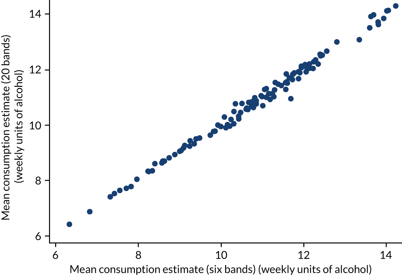
FIGURE 27.
Robustness: excluding GOR and mortality.
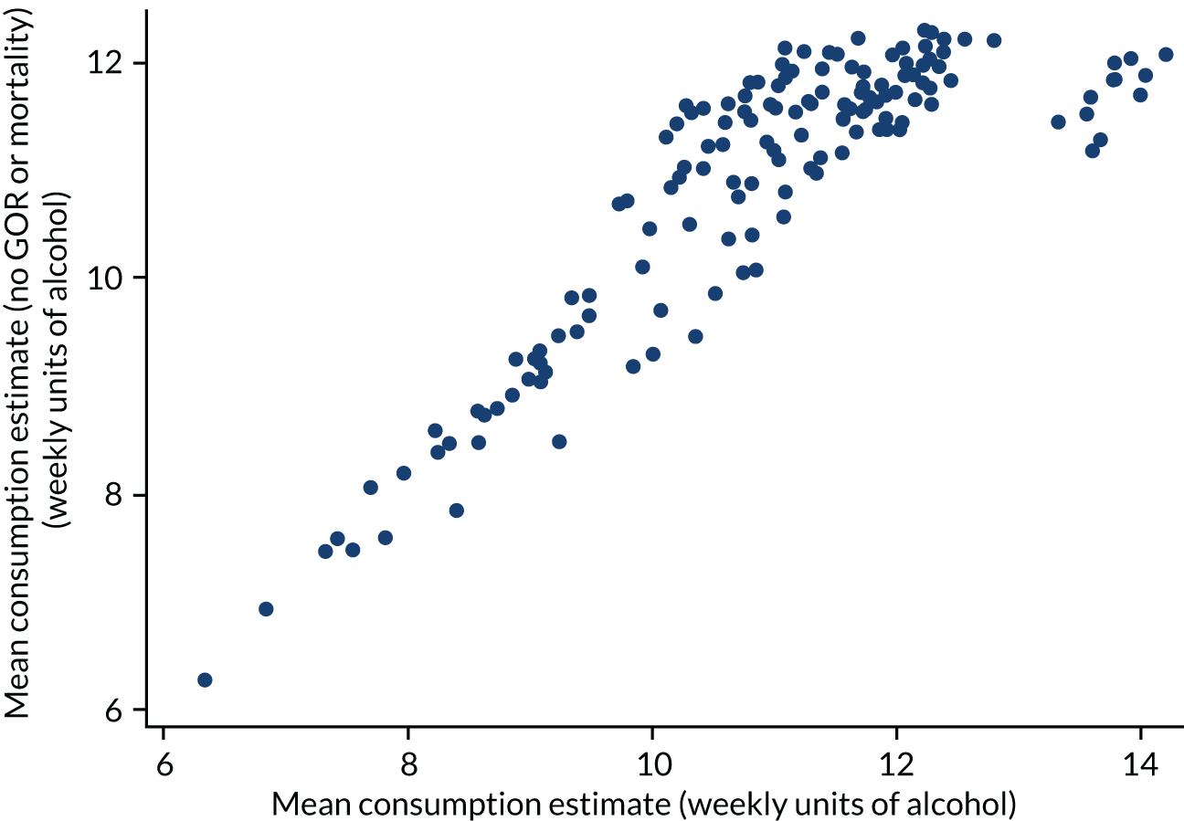
Appendix 2 Assumptions around the strengths of products used to derive price per unit in the Living Costs and Food Survey
| LCFS product description | Location | Alcohol by volume (%) | SAPM beverage category |
|---|---|---|---|
| Beer | Household | 4.0 | Off-trade beer |
| Lagers and continental beer | Household | 3.9 | Off-trade beer |
| Ciders and perry | Household | 4.8 | Off-trade cider |
| Champagne, sparkling wine and wine with mixer | Household | 11.4 | Off-trade wine |
| Table wine | Household | 12.8 | Off-trade wine |
| Spirits with mixer | Household | 7.4 | Off-trade spirits |
| Fortified wine | Household | 14.5 | Off-trade wine |
| Spirits | Household | 40.2 | Off-trade spirits |
| Liqueurs and cocktails | Household | 33.8 | Off-trade spirits |
| Alcopops | Household | 4.7 | Off-trade RTDs |
| Spirits | Eating out | 42.3 | On-trade spirits |
| Liqueurs | Eating out | 30.3 | On-trade spirits |
| Cocktails | Eating out | 13.4 | On-trade spirits |
| Spirits or liqueurs with mixer | Eating out | 7.8 | On-trade spirits |
| Wine (not sparkling) | Eating out | 11.3 | On-trade wine |
| Sparkling wine and wine with mixer | Eating out | 9.6 | On-trade wine |
| Fortified wine | Eating out | 17.5 | On-trade wine |
| Cider or perry | Eating out | 4.8 | On-trade cider |
| Alcopops | Eating out | 4.7 | On-trade RTDs |
| Bitter | Eating out | 4.3 | On-trade beer |
| Lager or other beers | Eating out | 5.1 | On-trade beer |
| Round of drinks, alcohol not otherwise specified | Eating out | 4.9 | On-trade beer |
Appendix 3 Regression results for price distributions
| Predictor variables | Beer | Cider | Wine | Spirits | RTDs |
|---|---|---|---|---|---|
| Price per unit of alcohol band | |||||
| 18–24 male | 0.000 | 0.000 | 0.000 | 0.000 | 0.000 |
| (.) | (.) | (.) | (.) | (.) | |
| 18–24 female | –0.446** | 0.526 | 0.933** | 0.014 | 0.130 |
| (0.150) | (0.276) | (0.301) | (0.195) | (0.732) | |
| 25–34 male | 0.463*** | 0.956*** | 1.798*** | 0.743*** | 0.780 |
| (0.076) | (0.205) | (0.285) | (0.172) | (0.543) | |
| 25–34 female | 0.463*** | 0.671* | 1.330*** | 0.890*** | 1.261 |
| (0.124) | (0.272) | (0.288) | (0.198) | (0.846) | |
| 35–54 male | 0.541*** | 0.499** | 1.732*** | 0.238 | 0.998* |
| (0.065) | (0.168) | (0.261) | (0.154) | (0.465) | |
| 35–54 female | 0.254* | 0.320 | 1.508*** | 0.643** | 0.841 |
| (0.099) | (0.249) | (0.281) | (0.204) | (0.755) | |
| ≥ 55 male | 0.216*** | 0.136 | 1.705*** | 0.746*** | 0.102 |
| (0.063) | (0.174) | (0.259) | (0.144) | (0.592) | |
| ≥ 55 female | 0.332** | 0.261 | 1.611*** | 0.539* | 1.223 |
| (0.102) | (0.291) | (0.281) | (0.230) | (1.097) | |
| Lowest income quintile | 0.000 | 0.000 | 0.000 | 0.000 | 0.000 |
| (.) | (.) | (.) | (.) | (.) | |
| Income quintile 2 | 0.119* | 0.023 | –0.301* | –0.438** | 0.120 |
| (0.056) | (0.180) | (0.127) | (0.155) | (0.557) | |
| Income quintile 3 | 0.445*** | 0.392* | 0.249* | –0.170 | –0.723 |
| (0.054) | (0.173) | (0.120) | (0.142) | (0.570) | |
| Income quintile 4 | 0.537*** | 0.332* | 0.300** | 0.560*** | –1.167* |
| (0.052) | (0.164) | (0.114) | (0.147) | (0.594) | |
| Highest income quintile | 0.962*** | 0.715*** | 0.612*** | 0.482** | –0.026 |
| (0.053) | (0.170) | (0.111) | (0.148) | (0.577) | |
| Moderate drinker | 0.000 | 0.000 | 0.000 | 0.000 | 0.000 |
| (.) | (.) | (.) | (.) | (.) | |
| Increasing-risk drinker | –0.174** | 0.117 | –0.176 | –0.995*** | –0.622 |
| (0.060) | (0.168) | (0.093) | (0.139) | (0.469) | |
| High-risk drinker | –0.349*** | –0.440** | –0.605*** | –1.511*** | –0.117 |
| (0.057) | (0.160) | (0.085) | (0.135) | (0.424) | |
| Outlet density | –0.000 | –0.001 | 0.005*** | –0.002 | 0.029* |
| (0.001) | (0.003) | (0.001) | (0.002) | (0.013) | |
| Alcohol-attributable hospitalisations | –0.001*** | –0.001 | –0.001** | 0.002*** | 0.001 |
| (0.000) | (0.000) | (0.000) | (0.000) | (0.002) | |
| Average house price | 0.003*** | 0.002* | 0.001* | 0.003*** | –0.002 |
| (0.000) | (0.001) | (0.000) | (0.001) | (0.002) | |
| cut1 | |||||
| _cons | –7.347*** | –4.717*** | –6.160*** | –3.548*** | –3.745 |
| (0.392) | (0.623) | (0.645) | (0.470) | (1.936) | |
| cut2 | |||||
| _cons | –5.206*** | –4.203*** | –3.534*** | –2.836*** | –2.194 |
| (0.212) | (0.597) | (0.413) | (0.454) | (1.842) | |
| cut3 | |||||
| _cons | –4.928*** | –3.567*** | –3.191*** | –1.851*** | –2.128 |
| (0.204) | (0.578) | (0.407) | (0.444) | (1.840) | |
| cut4 | |||||
| _cons | –4.421*** | –3.467*** | –2.927*** | –1.795*** | –2.005 |
| (0.193) | (0.576) | (0.404) | (0.444) | (1.838) | |
| cut5 | |||||
| _cons | –3.970*** | –3.012*** | –2.752*** | –1.575*** | –1.948 |
| (0.187) | (0.568) | (0.402) | (0.443) | (1.836) | |
| cut6 | |||||
| _cons | –3.705*** | –2.850*** | –2.452*** | –1.484*** | –0.485 |
| (0.184) | (0.567) | (0.400) | (0.443) | (1.828) | |
| cut7 | |||||
| _cons | –3.301*** | –2.580*** | –1.720*** | –1.311** | –0.463 |
| (0.181) | (0.564) | (0.396) | (0.442) | (1.828) | |
| cut8 | |||||
| _cons | –3.107*** | –2.397*** | –1.558*** | –0.892* | –0.338 |
| (0.180) | (0.563) | (0.396) | (0.441) | (1.828) | |
| cut9 | |||||
| _cons | –2.954*** | –2.341*** | –1.358*** | –0.853 | –0.317 |
| (0.180) | (0.563) | (0.396) | (0.441) | (1.828) | |
| cut10 | |||||
| _cons | –2.803*** | –2.121*** | –0.932* | –0.792 | –0.277 |
| (0.179) | (0.561) | (0.395) | (0.441) | (1.828) | |
| cut11 | |||||
| _cons | –2.624*** | –1.965*** | –0.775* | –0.694 | –0.238 |
| (0.178) | (0.561) | (0.395) | (0.440) | (1.828) | |
| cut12 | |||||
| _cons | –2.300*** | –1.759** | –0.608 | –0.669 | 0.087 |
| (0.178) | (0.560) | (0.395) | (0.440) | (1.829) | |
| cut13 | |||||
| _cons | –2.098*** | –1.559** | –0.481 | –0.502 | 0.137 |
| (0.177) | (0.559) | (0.395) | (0.440) | (1.830) | |
| cut14 | |||||
| _cons | –1.682*** | –1.291* | –0.378 | –0.433 | 0.296 |
| (0.176) | (0.558) | (0.395) | (0.440) | (1.831) | |
| cut15 | |||||
| _cons | –1.479*** | –1.046 | –0.274 | –0.374 | 0.357 |
| (0.176) | (0.558) | (0.395) | (0.440) | (1.832) | |
| cut16 | |||||
| _cons | –1.094*** | –0.808 | –0.248 | –0.347 | 0.402 |
| (0.176) | (0.557) | (0.395) | (0.440) | (1.832) | |
| cut17 | |||||
| _cons | –0.901*** | –0.679 | –0.137 | –0.326 | 0.431 |
| (0.175) | (0.557) | (0.395) | (0.440) | (1.832) | |
| cut18 | |||||
| _cons | –0.618*** | –0.115 | –0.065 | –0.290 | 0.939 |
| (0.175) | (0.556) | (0.395) | (0.440) | (1.836) | |
| cut19 | |||||
| _cons | –0.261 | 0.034 | 0.054 | –0.212 | 1.092 |
| (0.175) | (0.556) | (0.395) | (0.439) | (1.837) | |
| cut20 | |||||
| _cons | 0.127 | 0.332 | 0.130 | –0.192 | 1.194 |
| (0.175) | (0.556) | (0.395) | (0.439) | (1.837) | |
| cut21 | |||||
| _cons | 0.323 | 0.603 | 0.384 | –0.105 | 1.238 |
| (0.175) | (0.556) | (0.395) | (0.439) | (1.838) | |
| cut22 | |||||
| _cons | 0.637*** | 0.876 | 0.499 | 0.068 | 1.253 |
| (0.175) | (0.556) | (0.395) | (0.439) | (1.838) | |
| cut23 | |||||
| _cons | 1.065*** | 1.309* | 0.599 | 0.089 | 1.848 |
| (0.175) | (0.557) | (0.394) | (0.439) | (1.841) | |
| cut24 | |||||
| _cons | 1.339*** | 1.479** | 0.666 | 0.120 | 1.965 |
| (0.175) | (0.558) | (0.394) | (0.439) | (1.841) | |
| cut25 | |||||
| _cons | 1.634*** | 1.627** | 0.835* | 0.176 | 2.178 |
| (0.176) | (0.558) | (0.394) | (0.439) | (1.841) | |
| cut26 | |||||
| _cons | 1.983*** | 1.976*** | 0.923* | 0.225 | 2.292 |
| (0.176) | (0.560) | (0.394) | (0.439) | (1.841) | |
| cut27 | |||||
| _cons | 2.248*** | 2.070*** | 1.123** | 0.267 | 2.413 |
| (0.176) | (0.560) | (0.394) | (0.439) | (1.841) | |
| cut28 | |||||
| _cons | 2.617*** | 2.231*** | 1.197** | 0.307 | 2.967 |
| (0.177) | (0.560) | (0.394) | (0.439) | (1.841) | |
| cut29 | |||||
| _cons | 2.767*** | 2.297*** | 1.318*** | 0.374 | |
| (0.177) | (0.561) | (0.394) | (0.439) | ||
| cut30 | |||||
| _cons | 3.005*** | 2.389*** | 1.401*** | 0.397 | |
| (0.178) | (0.561) | (0.394) | (0.439) | ||
| cut31 | |||||
| _cons | 3.118*** | 2.443*** | 1.744*** | 0.427 | |
| (0.178) | (0.561) | (0.394) | (0.439) | ||
| cut32 | |||||
| _cons | 3.489*** | 2.518*** | 1.783*** | 0.444 | |
| (0.179) | (0.561) | (0.394) | (0.439) | ||
| cut33 | |||||
| _cons | 3.588*** | 2.595*** | 1.871*** | 0.609 | |
| (0.180) | (0.562) | (0.394) | (0.439) | ||
| cut34 | |||||
| _cons | 3.741*** | 2.665*** | 2.013*** | 0.612 | |
| (0.180) | (0.562) | (0.394) | (0.439) | ||
| cut35 | |||||
| _cons | 3.832*** | 2.754*** | 2.076*** | 0.629 | |
| (0.181) | (0.563) | (0.395) | (0.439) | ||
| cut36 | |||||
| _cons | 4.113*** | 2.855*** | 2.283*** | 0.662 | |
| (0.182) | (0.563) | (0.395) | (0.439) | ||
| cut37 | |||||
| _cons | 4.268*** | 2.928*** | 2.357*** | 0.717 | |
| (0.183) | (0.563) | (0.395) | (0.439) | ||
| cut38 | |||||
| _cons | 4.341*** | 3.055*** | 2.543*** | 0.743 | |
| (0.184) | (0.564) | (0.395) | (0.439) | ||
| cut39 | |||||
| _cons | 4.384*** | 3.321*** | 2.628*** | 0.806 | |
| (0.184) | (0.566) | (0.395) | (0.439) | ||
| cut40 | |||||
| _cons | 4.504*** | 3.346*** | 2.691*** | 0.826 | |
| (0.185) | (0.567) | (0.395) | (0.439) | ||
| cut41 | |||||
| _cons | 4.726*** | 3.430*** | 2.836*** | 0.975* | |
| (0.187) | (0.567) | (0.395) | (0.439) | ||
| cut42 | |||||
| _cons | 4.775*** | 3.760*** | 3.051*** | 0.996* | |
| (0.187) | (0.571) | (0.395) | (0.439) | ||
| cut43 | |||||
| _cons | 4.903*** | 3.860*** | 3.107*** | 1.011* | |
| (0.189) | (0.573) | (0.396) | (0.439) | ||
| cut44 | |||||
| _cons | 5.075*** | 3.192*** | 1.142** | ||
| (0.191) | (0.396) | (0.440) | |||
| cut45 | |||||
| _cons | 5.167*** | 3.425*** | 1.166** | ||
| (0.192) | (0.396) | (0.440) | |||
| cut46 | |||||
| _cons | 3.492*** | 1.204** | |||
| (0.396) | (0.440) | ||||
| cut47 | |||||
| _cons | 3.576*** | 1.229** | |||
| (0.396) | (0.440) | ||||
| cut48 | |||||
| _cons | 3.607*** | 1.272** | |||
| (0.396) | (0.440) | ||||
| cut49 | |||||
| _cons | 1.310** | ||||
| (0.440) | |||||
| N | 15,180 | 1654 | 5515 | 2731 | 168 |
| Predictor variables | Beer | Cider | Wine | Spirits | RTDs |
|---|---|---|---|---|---|
| Price per unit of alcohol band | |||||
| 18–24 male | 0.000 | 0.000 | 0.000 | 0.000 | 0.000 |
| (.) | (.) | (.) | (.) | (.) | |
| 18–24 female | –0.402 | 0.229 | 0.715** | 0.573 | 0.683 |
| (0.220) | (0.313) | (0.271) | (0.362) | (0.863) | |
| 25–34 male | –0.225 | –0.349 | 0.344 | 0.464 | –0.347 |
| (0.133) | (0.246) | (0.244) | (0.293) | (0.698) | |
| 25–34 female | –0.462** | –0.124 | 0.297 | 0.673* | 0.957 |
| (0.161) | (0.270) | (0.245) | (0.322) | (0.826) | |
| 35–54 male | –0.072 | –0.657** | 0.198 | –0.256 | –0.416 |
| (0.125) | (0.219) | (0.231) | (0.262) | (0.674) | |
| 35–54 female | –0.211 | –0.885*** | 0.117 | 0.007 | 0.458 |
| (0.145) | (0.252) | (0.237) | (0.286) | (0.797) | |
| ≥ 55 male | 0.079 | –1.148*** | 0.206 | –0.318 | 0.262 |
| (0.127) | (0.225) | (0.231) | (0.257) | (0.681) | |
| ≥ 55 female | –0.319* | –1.143*** | 0.027 | –0.100 | 0.463 |
| (0.148) | (0.259) | (0.237) | (0.285) | (0.782) | |
| Lowest income quintile | 0.000 | 0.000 | 0.000 | 0.000 | 0.000 |
| (.) | (.) | (.) | (.) | (.) | |
| Income quintile 2 | 0.255*** | 0.293** | –0.087 | 0.239* | 0.740* |
| (0.067) | (0.112) | (0.062) | (0.109) | (0.316) | |
| Income quintile 3 | 0.409*** | 0.503*** | 0.229*** | 0.237* | 1.050** |
| (0.064) | (0.115) | (0.057) | (0.110) | (0.328) | |
| Income quintile 4 | 0.393*** | 0.868*** | 0.382*** | 0.359*** | 0.276 |
| (0.061) | (0.110) | (0.055) | (0.106) | (0.311) | |
| Highest income quintile | 0.916*** | 1.083*** | 1.055*** | 0.656*** | 1.061** |
| (0.064) | (0.116) | (0.055) | (0.105) | (0.331) | |
| Moderate drinker | 0.000 | 0.000 | 0.000 | 0.000 | 0.000 |
| (.) | (.) | (.) | (.) | (.) | |
| Increasing-risk drinker | –0.781*** | –0.706*** | –0.215* | –0.382 | 0.531 |
| (0.118) | (0.171) | (0.087) | (0.328) | (0.358) | |
| High-risk drinker | –1.430*** | –1.472*** | –0.508*** | –0.891** | –0.320 |
| (0.112) | (0.159) | (0.081) | (0.317) | (0.297) | |
| Outlet density | –0.001 | 0.007* | –0.000 | –0.000 | –0.005 |
| (0.001) | (0.003) | (0.001) | (0.002) | (0.007) | |
| Alcohol-attributable hospitalisations | –0.001** | –0.001*** | 0.000 | 0.001* | 0.002 |
| (0.000) | (0.000) | (0.000) | (0.000) | (0.001) | |
| Average house price | 0.001* | –0.001 | 0.002*** | 0.001** | 0.002 |
| (0.000) | (0.001) | (0.000) | (0.000) | (0.002) | |
| cut1 | |||||
| _cons | –7.596*** | –7.697*** | –5.293*** | –8.767*** | –2.984 |
| (0.358) | (0.521) | (0.329) | (1.646) | (1.678) | |
| cut2 | |||||
| _cons | –7.333*** | –7.354*** | –5.030*** | –6.178*** | –2.419 |
| (0.340) | (0.506) | (0.321) | (0.695) | (1.620) | |
| cut3 | |||||
| _cons | –6.030*** | –6.573*** | –3.992*** | –4.810*** | –1.518 |
| (0.292) | (0.485) | (0.303) | (0.590) | (1.574) | |
| cut4 | |||||
| _cons | –5.771*** | –4.770*** | –3.587*** | –4.425*** | –1.120 |
| (0.288) | (0.469) | (0.299) | (0.578) | (1.564) | |
| cut5 | |||||
| _cons | –4.706*** | –3.643*** | –3.060*** | –3.918*** | –0.490 |
| (0.278) | (0.467) | (0.296) | (0.567) | (1.553) | |
| cut6 | |||||
| _cons | –3.452*** | –2.931*** | –2.460*** | –3.048*** | 0.280 |
| (0.274) | (0.465) | (0.294) | (0.557) | (1.545) | |
| cut7 | |||||
| _cons | –2.413*** | –2.290*** | –1.516*** | –2.291*** | 0.962 |
| (0.273) | (0.463) | (0.293) | (0.554) | (1.541) | |
| cut8 | |||||
| _cons | –1.849*** | –1.685*** | –0.525 | –0.889 | 1.311 |
| (0.272) | (0.463) | (0.292) | (0.551) | (1.539) | |
| cut9 | |||||
| _cons | –1.239*** | –1.417** | 0.267 | 0.068 | 1.644 |
| (0.272) | (0.463) | (0.292) | (0.551) | (1.539) | |
| cut10 | |||||
| _cons | –0.755** | –1.075* | 0.702* | 0.748 | 1.969 |
| (0.272) | (0.463) | (0.292) | (0.552) | (1.541) | |
| cut11 | |||||
| _cons | –0.310 | –0.724 | 1.537*** | 1.236* | 2.288 |
| (0.272) | (0.463) | (0.292) | (0.552) | (1.542) | |
| cut12 | |||||
| _cons | 0.047 | –0.506 | 1.874*** | 1.619** | 2.732 |
| (0.272) | (0.463) | (0.292) | (0.552) | (1.545) | |
| cut13 | |||||
| _cons | 0.371 | –0.040 | 2.349*** | 1.871*** | 3.075* |
| (0.272) | (0.464) | (0.293) | (0.552) | (1.546) | |
| cut14 | |||||
| _cons | 0.666* | 0.365 | 2.595*** | 2.143*** | 3.542* |
| (0.272) | (0.465) | (0.293) | (0.552) | (1.548) | |
| cut15 | |||||
| _cons | 1.036*** | 0.747 | 2.959*** | 2.334*** | 3.725* |
| (0.272) | (0.466) | (0.293) | (0.553) | (1.550) | |
| cut16 | |||||
| _cons | 1.236*** | 1.048* | 3.195*** | 2.606*** | 4.164** |
| (0.273) | (0.468) | (0.293) | (0.553) | (1.553) | |
| cut17 | |||||
| _cons | 1.684*** | 1.543** | 3.292*** | 2.752*** | 4.464** |
| (0.274) | (0.473) | (0.294) | (0.554) | (1.554) | |
| cut18 | |||||
| _cons | 1.954*** | 1.735*** | 3.581*** | 2.998*** | 4.726** |
| (0.275) | (0.476) | (0.294) | (0.554) | (1.555) | |
| cut19 | |||||
| _cons | 2.224*** | 2.357*** | 3.727*** | 3.103*** | 4.852** |
| (0.276) | (0.490) | (0.294) | (0.555) | (1.556) | |
| cut20 | |||||
| _cons | 2.554*** | 2.693*** | 3.926*** | 3.319*** | 4.895** |
| (0.279) | (0.502) | (0.295) | (0.555) | (1.557) | |
| cut21 | |||||
| _cons | 2.829*** | 2.903*** | 4.007*** | 3.516*** | 4.964** |
| (0.281) | (0.512) | (0.295) | (0.556) | (1.557) | |
| cut22 | |||||
| _cons | 2.952*** | 3.464*** | 4.268*** | 3.772*** | 5.111** |
| (0.282) | (0.548) | (0.296) | (0.558) | (1.559) | |
| cut23 | |||||
| _cons | 3.123*** | 3.982*** | 4.323*** | 4.056*** | 5.459*** |
| (0.285) | (0.602) | (0.296) | (0.561) | (1.563) | |
| cut24 | |||||
| _cons | 3.193*** | 4.466*** | 4.429*** | 4.255*** | 5.838*** |
| (0.286) | (0.676) | (0.296) | (0.563) | (1.569) | |
| cut25 | |||||
| _cons | 3.284*** | 4.535*** | 4.510*** | 4.425*** | 6.046*** |
| (0.287) | (0.689) | (0.296) | (0.565) | (1.574) | |
| cut26 | |||||
| _cons | 3.380*** | 4.869*** | 4.678*** | 4.677*** | 6.308*** |
| (0.289) | (0.761) | (0.297) | (0.569) | (1.582) | |
| cut27 | |||||
| _cons | 3.630*** | 5.953*** | 4.744*** | 4.823*** | 6.504*** |
| (0.294) | (1.140) | (0.297) | (0.572) | (1.589) | |
| cut28 | |||||
| _cons | 3.792*** | 6.840*** | 4.852*** | 5.286*** | 6.540*** |
| (0.298) | (1.690) | (0.298) | (0.585) | (1.591) | |
| cut29 | |||||
| _cons | 3.953*** | 7.177*** | 4.888*** | 5.379*** | 6.620*** |
| (0.303) | (1.978) | (0.298) | (0.588) | (1.594) | |
| cut30 | |||||
| _cons | 4.132*** | 5.005*** | 5.707*** | 6.839*** | |
| (0.309) | (0.299) | (0.602) | (1.605) | ||
| cut31 | |||||
| _cons | 4.308*** | 5.123*** | 5.866*** | 7.499*** | |
| (0.315) | (0.299) | (0.610) | (1.654) | ||
| cut32 | |||||
| _cons | 4.336*** | 5.290*** | 6.117*** | 7.798*** | |
| (0.317) | (0.301) | (0.626) | (1.688) | ||
| cut33 | |||||
| _cons | 4.386*** | 5.347*** | 6.180*** | 8.083*** | |
| (0.319) | (0.301) | (0.631) | (1.731) | ||
| cut34 | |||||
| _cons | 4.443*** | 5.420*** | 6.257*** | 8.699*** | |
| (0.322) | (0.302) | (0.637) | (1.870) | ||
| cut35 | |||||
| _cons | 4.596*** | 5.518*** | 6.614*** | 11.099** | |
| (0.329) | (0.302) | (0.670) | (3.795) | ||
| cut36 | |||||
| _cons | 4.780*** | 5.561*** | 6.872*** | ||
| (0.340) | (0.303) | (0.702) | |||
| cut37 | |||||
| _cons | 4.852*** | 5.590*** | 7.271*** | ||
| (0.345) | (0.303) | (0.765) | |||
| cut38 | |||||
| _cons | 4.895*** | 5.605*** | 7.339*** | ||
| (0.348) | (0.303) | (0.778) | |||
| cut39 | |||||
| _cons | 4.932*** | 5.730*** | 7.504*** | ||
| (0.350) | (0.305) | (0.813) | |||
| cut40 | |||||
| _cons | 5.019*** | 5.796*** | 7.567*** | ||
| (0.357) | (0.306) | (0.827) | |||
| cut41 | |||||
| _cons | 5.167*** | 5.854*** | 7.739*** | ||
| (0.369) | (0.306) | (0.869) | |||
| cut42 | |||||
| _cons | 5.181*** | 5.879*** | 8.445*** | ||
| (0.370) | (0.307) | (1.104) | |||
| cut43 | |||||
| _cons | 5.202*** | 6.065*** | 8.546*** | ||
| (0.372) | (0.309) | (1.147) | |||
| cut44 | |||||
| _cons | 5.267*** | 6.069*** | 8.977*** | ||
| (0.377) | (0.309) | (1.365) | |||
| cut45 | |||||
| _cons | 5.429*** | 6.080*** | |||
| (0.393) | (0.310) | ||||
| cut46 | |||||
| _cons | 5.651*** | 6.146*** | |||
| (0.418) | (0.311) | ||||
| cut47 | |||||
| _cons | 5.681*** | 6.225*** | |||
| (0.422) | (0.312) | ||||
| cut48 | |||||
| _cons | 5.707*** | 6.244*** | |||
| (0.425) | (0.312) | ||||
| N | 9033 | 2781 | 16,628 | 3414 | 424 |
Appendix 4 Evidence briefings for the North East Government Office Region as a whole and for one example upper-tier local authority (Redcar and Cleveland)
The University of Sheffield logo has been reproduced with permission (University of Sheffield, 2021, personal communication).
Appendix 5 Three PowerPoint slides from the evidence asset band for national results for England
At a national level, we estimate that there are currently almost 10,000 people per annum dying as a result of alcohol consumption (Figure 28). We estimate that > 650,000 hospital admissions are caused by alcohol each year. This results in an annual cost to the NHS of > £2.8B per year. We also estimate that nationally there are around 2,300,000 crimes per year caused by alcohol, including over half a million thefts or robberies and over half a million violent incidents.
FIGURE 28.
Scale of the problem: PowerPoint evidence asset slide for England.
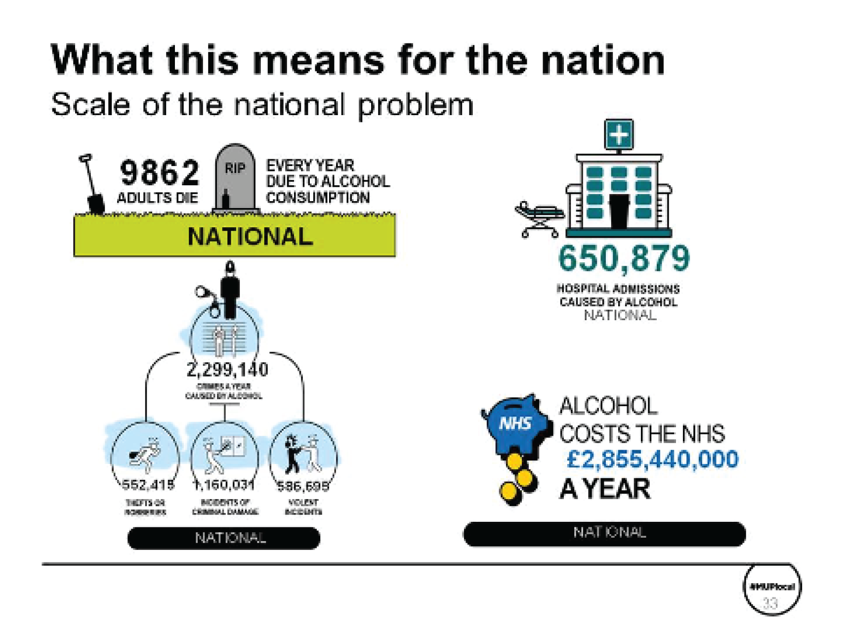
The burden of alcohol is not just in the harm done to the individual drinker. Children are also affected; the CIN statistics produced by the government show that ≈ 82,000 children were in contact with social care services over 1 year, with alcohol identified as one of the contributory factors (Figure 29) (characteristics of children in need: 2015 to 2016, see column F in table C379).
FIGURE 29.
Scale of the problem: PowerPoint evidence asset slide on workplace and children’s social care.
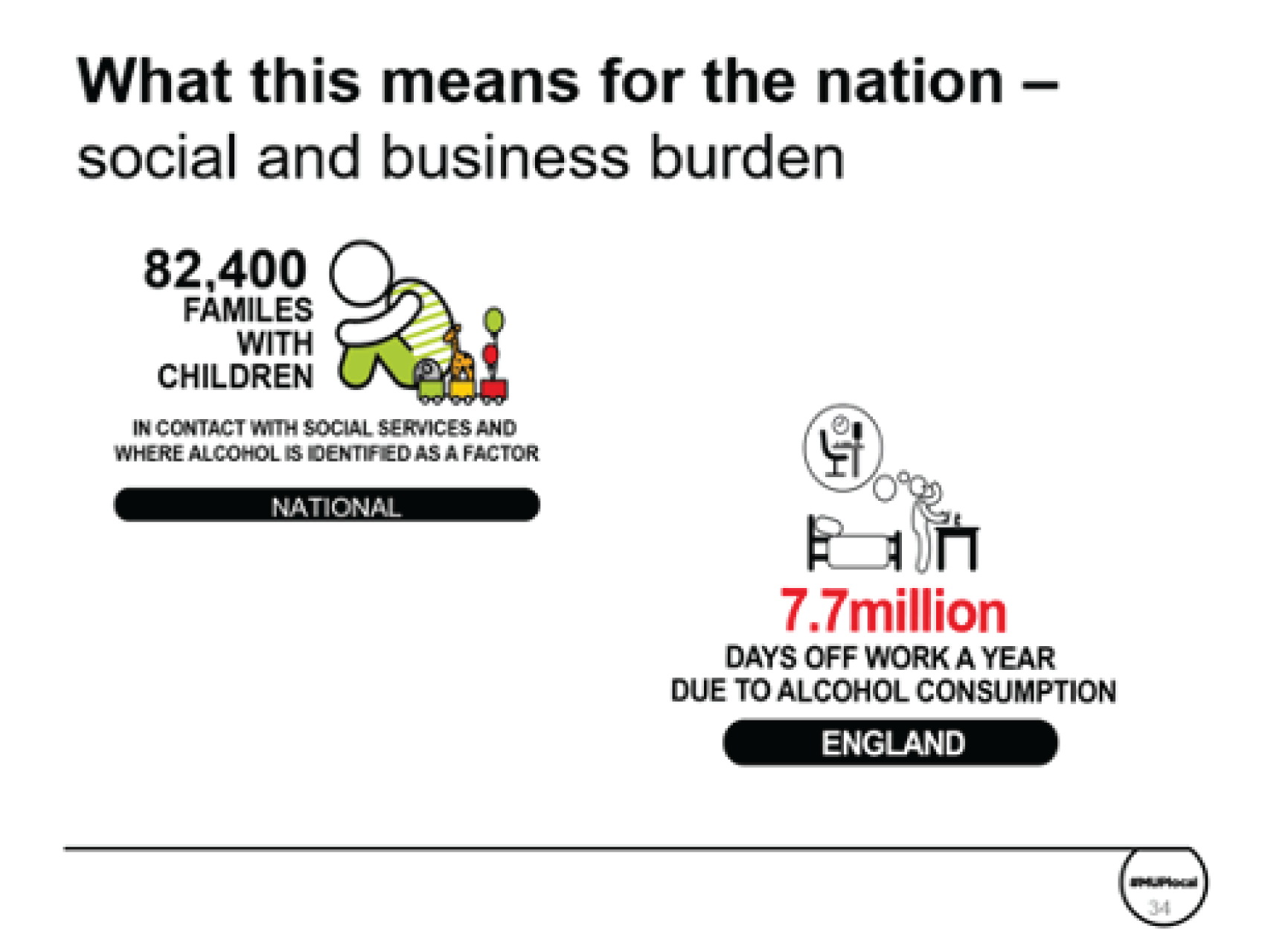
Figure 30 presents the potential benefits of a 50p MUP for England.
FIGURE 30.
PowerPoint evidence asset slide outlining the impact of a 50p MUP for England.
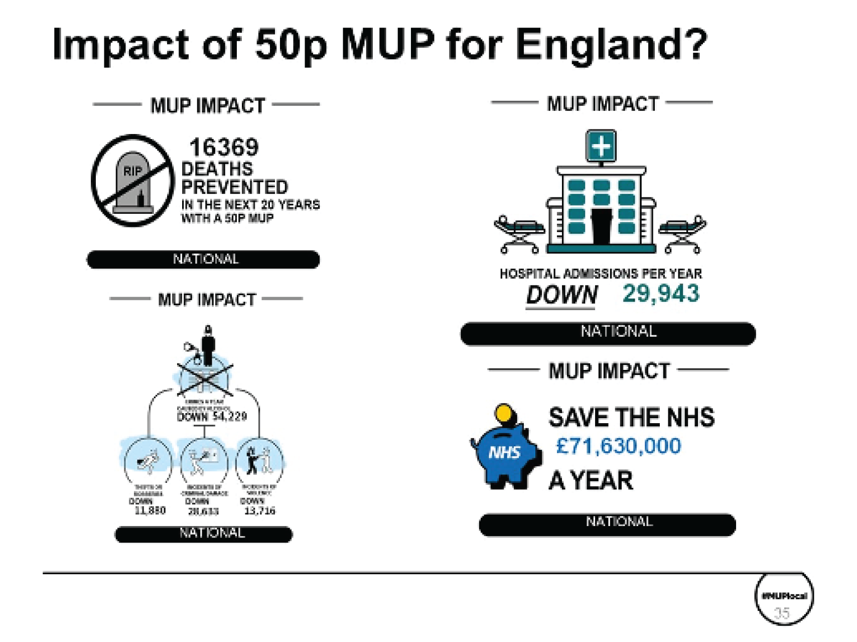
Appendix 6 Summary results tables for the North East region
| Statistic of interest | North East UTLAs | North West | North East | England | |||||||||||
|---|---|---|---|---|---|---|---|---|---|---|---|---|---|---|---|
| County Durham | Darlington | Gateshead | Hartlepool | Middlesbrough | Newcastle | Northumberland | North Tyneside | Redcar | Stockton | South Tyneside | Sunderland | ||||
| Adult population (aged ≥ 18 years) (n) | 408,853 | 81,138 | 157,176 | 71,266 | 105,634 | 228,107 | 250,446 | 228,107 | 105,523 | 148,697 | 116,834 | 218,217 | 5,500,855 | 2,050,703 | 41,614,894 |
| Mean weekly alcohol consumption (units) | |||||||||||||||
| Per drinker | 16.3 | 16.1 | 16.9 | 16.8 | 17.3 | 16.9 | 16.0 | 11.8 | 11.5 | 16.0 | 16.1 | 16.3 | 14.4 | 16.4 | 13.3 |
| Moderate drinkers | 4.4 | 4.4 | 4.4 | 4.3 | 4.2 | 4.4 | 4.4 | 4.4 | 4.4 | 4.4 | 4.2 | 4.3 | 4.3 | 4.4 | 4.3 |
| Increasing-risk drinkers | 25.0 | 24.9 | 25.2 | 25.4 | 25.6 | 25.7 | 25.1 | 25.7 | 25.3 | 25.1 | 24.9 | 25.1 | 24.8 | 25.2 | 24.7 |
| High-risk drinkers | 80.0 | 78.9 | 80.4 | 79.7 | 79.7 | 77.1 | 76.7 | 77.1 | 78.2 | 77.5 | 81.5 | 80.8 | 77.5 | 79.0 | 75.6 |
| Abstaining (%) | 14.7 | 14.1 | 15.4 | 16.1 | 20.7 | 19.4 | 13.5 | 19.4 | 15.2 | 14.8 | 16.7 | 16.4 | 17.9 | 15.7 | 17.1 |
| Moderate drinkers (%) | 54.9 | 55.3 | 53.6 | 53.1 | 49.8 | 50.2 | 55.1 | 50.2 | 53.6 | 54.6 | 54.8 | 54.0 | 55.5 | 53.8 | 57.4 |
| Increasing-risk drinkers (%) | 23.4 | 23.6 | 23.5 | 23.4 | 22.0 | 23.5 | 24.7 | 23.5 | 23.9 | 23.7 | 21.5 | 22.5 | 21.2 | 23.4 | 21.0 |
| High-risk drinkers (%) | 7.0 | 7.0 | 7.4 | 7.3 | 7.5 | 7.0 | 6.8 | 7.0 | 7.3 | 6.8 | 7.0 | 7.0 | 5.3 | 7.1 | 4.5 |
| Alcohol-related deaths per year (n) | 137 | 28 | 58 | 29 | 40 | 74 | 82 | 59 | 35 | 52 | 50 | 89 | 1791 | 697 | 9862 |
| Alcohol-related mortality per 100,000 adult population | 33.5 | 34.8 | 37.1 | 40.9 | 38.1 | 32.3 | 32.7 | 25.7 | 33.2 | 34.9 | 42.4 | 40.6 | 32.6 | 34.0 | 23.7 |
| Alcohol-attributable admissions per year (n) | 8252 | 1625 | 3217 | 1706 | 2600 | 4266 | 4948 | 3482 | 2409 | 3089 | 2795 | 4653 | 108,403 | 41,159 | 650,879 |
| Alcohol-attributable admissions per 100,000 adult population | 2018.3 | 2002.6 | 2046.7 | 2393.5 | 2461.1 | 1870.3 | 1975.9 | 1526.4 | 2282.8 | 2077.3 | 2392.7 | 2132.3 | 1970.7 | 2007.1 | 1563.0 |
| Alcohol-attributable crimes per year (n) | 22,134 | 5402 | 8617 | 5196 | 9988 | 15,684 | 10,865 | 7494 | 7757 | 8714 | 7358 | 13,739 | 341,202 | 125,625 | 2,299,140 |
| Alcohol-attributable crimes per 100,000 adult population | 5413.6 | 6657.7 | 5482.5 | 7290.4 | 9455.3 | 6875.7 | 4338.2 | 3285.4 | 7351.4 | 5860.4 | 6297.7 | 6295.8 | 6202.7 | 6125.9 | 5521.2 |
| Alcohol-attributable NHS cost per year (£000,000) | 36.9 | 7.3 | 15.0 | 7.6 | 11.9 | 19.6 | 21.4 | 15.6 | 10.7 | 13.4 | 12.1 | 20.6 | 504.6 | 185.5 | 2,855.4 |
| Mean annual expenditure on alcohol (£) | |||||||||||||||
| Per adult | 565 | 577 | 579 | 568 | 709 | 585 | 583 | 584 | 578 | 575 | 542 | 547 | 500 | 570 | 481 |
| Moderate drinkers | 207 | 215 | 207 | 201 | 281 | 217 | 216 | 216 | 207 | 214 | 198 | 198 | 203 | 208 | 208 |
| Increasing-risk drinkers | 1013 | 1027 | 1016 | 1020 | 1313 | 1077 | 1050 | 1075 | 1033 | 1043 | 995 | 993 | 1021 | 1028 | 1020 |
| High-risk drinkers | 2624 | 2651 | 2643 | 2599 | 2961 | 2589 | 2593 | 2586 | 2584 | 2615 | 2663 | 2616 | 2504 | 2616 | 2508 |
| Mean weekly consumption of alcohol (units) priced at < 50p per unit | |||||||||||||||
| Per adult | 6.8 | 6.4 | 7.1 | 7.1 | 7.5 | 6.7 | 6.2 | 6.7 | 6.9 | 6.3 | 6.9 | 698.9 | 5.5 | 6.5 | 5.4 |
| Moderate drinkers | 1.1 | 1.0 | 1.1 | 1.1 | 1.1 | 1.0 | 1.0 | 1.0 | 1.1 | 1.0 | 1.1 | 110.2 | 1.0 | 0.9 | 1.1 |
| Increasing-risk drinkers | 9.6 | 9.1 | 9.6 | 9.8 | 10.1 | 9.2 | 9.0 | 9.3 | 9.5 | 9.0 | 9.7 | 988.5 | 8.9 | 9.0 | 9.7 |
| High-risk drinkers | 42.6 | 40.4 | 42.1 | 42.5 | 42.6 | 39.1 | 39.0 | 38.9 | 41.1 | 39.3 | 43.3 | 4312.4 | 39.3 | 40.0 | 40.4 |
| Mean annual expenditure per adult (£) on alcohol priced at < 50p per unit | |||||||||||||||
| Per adult | 116.48 | 111.80 | 119.08 | 119.60 | 118.04 | 108.16 | 109.20 | 110.76 | 117.00 | 107.64 | 113.36 | 115.96 | 90.48 | 113.36 | 79.04 |
| Moderate drinkers | 22.36 | 21.32 | 22.36 | 22.36 | 22.36 | 19.76 | 20.80 | 21.32 | 21.84 | 20.80 | 22.36 | 22.88 | 21.32 | 21.84 | 19.24 |
| Increasing-risk drinkers | 194.48 | 185.64 | 192.92 | 198.64 | 202.28 | 187.20 | 184.08 | 183.04 | 192.92 | 183.04 | 195.00 | 198.12 | 176.80 | 190.84 | 170.04 |
| High-risk drinkers | 846.04 | 808.08 | 830.96 | 840.84 | 836.16 | 778.96 | 780.52 | 786.24 | 816.92 | 784.68 | 852.80 | 846.56 | 776.88 | 817.44 | 729.56 |
| Statistic of interest | North East UTLAs | North West | North East | England | |||||||||||
|---|---|---|---|---|---|---|---|---|---|---|---|---|---|---|---|
| County Durham | Darlington | Gateshead | Hartlepool | Middlesbrough | Newcastle | Northumberland | North Tyneside | Redcar | Stockton | South Tyneside | Sunderland | ||||
| Change in mean weekly units | |||||||||||||||
| All drinkers | –1.1 | –1.0 | –1.2 | –1.2 | –1.3 | –1.0 | –0.9 | –1.1 | –1.1 | –0.9 | –1.2 | –1.3 | –0.6 | –1.1 | –0.4 |
| Moderate drinkers | –0.1 | –0.1 | –0.1 | –0.1 | –0.1 | –0.1 | –0.1 | –0.1 | –0.1 | –0.1 | –0.1 | –0.1 | –0.1 | –0.1 | –0.1 |
| Increasing-risk drinkers | –1.6 | –1.4 | –1.9 | –1.8 | –2.1 | –1.7 | –1.4 | –1.8 | –1.6 | –1.5 | –1.9 | –2.0 | –1.1 | –1.7 | –0.9 |
| High-risk drinkers | –8.7 | –7.9 | –9.6 | –9.2 | –10.3 | –8.1 | –7.4 | –8.5 | –8.4 | –7.8 | –10.0 | –10.3 | –6.0 | –8.8 | –4.2 |
| Change in mean weekly alcohol consumption (%) | |||||||||||||||
| All drinkers | –6.5 | –5.9 | –7.3 | –7.0 | –7.7 | –6.0 | –5.6 | –9.1 | –9.3 | –5.9 | –7.4 | –7.8 | –4.3 | –6.6 | –3.6 |
| Moderate drinkers | –2.2 | –1.9 | –2.6 | –2.4 | –2.9 | –2.1 | –1.8 | –2.3 | –2.2 | –1.9 | –2.7 | –2.8 | –1.9 | –2.2 | –1.5 |
| Increasing-risk drinkers | –6.5 | –5.8 | –7.4 | –7.1 | –8.3 | –6.5 | –5.6 | –6.8 | –6.4 | –5.9 | –7.6 | –8.1 | –4.5 | –6.7 | –3.9 |
| High-risk drinkers | –10.9 | –10.0 | –11.9 | –11.6 | –12.9 | –10.5 | –9.7 | –11.0 | –10.8 | –10.1 | –12.3 | –12.8 | –7.7 | –11.1 | –5.6 |
| Change in alcohol-attributable deaths | |||||||||||||||
| Annual deaths reduction | –23 | –4 | –11 | –5 | –8 | –13 | –12 | –9 | –6 | –9 | –8 | –17 | –205 | –121 | –1024 |
| Reduction in deaths over 20-year horizon | –374 | –71 | –174 | –84 | –133 | –203 | –204 | –158 | –100 | –140 | –144 | –270 | –3332 | –1970 | –16,369 |
| Change in death rate per 100,000 adult population | –5.5 | –5.4 | –6.8 | –7.2 | –7.9 | –5.8 | –4.7 | –4.1 | –5.7 | –6.0 | –7.3 | –7.6 | –3.7 | –5.9 | –2.5 |
| Change in death rate (%) | –16.5 | –15.6 | –18.3 | –17.7 | –20.7 | –17.9 | –14.4 | –16.0 | –17.3 | –17.1 | –17.1 | –18.7 | –11.4 | –17.4 | –10.4 |
| Change in alcohol-attributable hospital admissions | |||||||||||||||
| Reduction in number of admissions per year | –589 | –115 | –283 | –135 | –256 | –398 | –296 | –258 | –171 | –235 | –222 | –415 | –5956 | –3255 | –29,943 |
| Reduction in admission rate per 100,000 adult population | –144.1 | –141.5 | –180.1 | –188.8 | –242.0 | –174.5 | –118.0 | –112.9 | –161.8 | –157.9 | –189.8 | –190.0 | –108.3 | –158.7 | –71.9 |
| Change in hospital admission rate (%) | –7.1 | –7.1 | –8.8 | –7.9 | –9.8 | –9.3 | –6.0 | –7.4 | –7.1 | –7.6 | –7.9 | –8.9 | –5.5 | –7.9 | –4.6 |
| Change in alcohol-attributable crimes | |||||||||||||||
| Reduction in number of crimes per year | –734 | –166 | –338 | –193 | –436 | –509 | –323 | –257 | –261 | –272 | –289 | –592 | –8528 | –4380 | –54,229 |
| Reduction in crime rate per 100,000 adult population | –179.5 | –204.5 | –215.2 | –270.8 | –412.9 | –223.1 | –129.0 | –112.7 | –246.9 | –183.1 | –247.1 | –271.5 | –155.0 | –213.6 | –130.2 |
| Change in crime rate (%) | –3.3 | –3.1 | –3.9 | –3.7 | –4.4 | –3.2 | –3.0 | –3.4 | –3.4 | –3.1 | –3.9 | –4.3 | –2.5 | –3.5 | –2.4 |
| Costs savings to NHS over 20 years | |||||||||||||||
| Reduction in annual NHS costs (£000,000) | –1.6 | –0.3 | –0.9 | –0.3 | –0.6 | –1.1 | –0.8 | –0.7 | –0.5 | –0.6 | –0.6 | –1.1 | –12.2 | –8.4 | –71.6 |
| Change in NHS costs (%) | –4.3 | –3.7 | –5.7 | –4.2 | –5.2 | –5.6 | –3.7 | –4.2 | –4.3 | –4.4 | –4.5 | –5.1 | –2.4 | –4.5 | –2.5 |
| Statistic of interest | North East UTLAs | North West | North East | England | |||||||||||
|---|---|---|---|---|---|---|---|---|---|---|---|---|---|---|---|
| County Durham | Darlington | Gateshead | Hartlepool | Middlesbrough | Newcastle | Northumberland | North Tyneside | Redcar | Stockton | South Tyneside | Sunderland | ||||
| Change in mean annual expenditure on alcohol (£) | |||||||||||||||
| Per drinker | 3.41 | 4.36 | –0.23 | 2.11 | –1.57 | 1.91 | 4.65 | 0.54 | 3.43 | 3.59 | 0.14 | –1.23 | 7.11 | 2.07 | 8.89 |
| Moderate drinkers | 2.46 | 2.55 | 1.98 | 2.38 | 1.89 | 2.05 | 2.57 | 1.83 | 2.47 | 2.35 | 2.06 | 1.94 | 2.34 | 2.25 | 2.53 |
| Increasing-risk drinkers | 4.01 | 6.15 | –2.07 | 1.93 | –4.80 | 0.98 | 6.40 | –1.46 | 4.16 | 4.66 | –1.16 | –4.06 | 10.99 | 1.93 | 14.82 |
| High-risk drinkers | 10.87 | 16.26 | –14.92 | 0.14 | –24.66 | 3.66 | 19.28 | –5.46 | 10.03 | 12.60 | –15.43 | –24.02 | 57.23 | 0.70 | 86.95 |
| Change in revenue to retailers (£000,000) | |||||||||||||||
| Off-trade | 5.72 | 1.09 | 2.06 | 1.00 | 1.37 | 2.78 | 3.29 | 2.68 | 1.47 | 1.88 | 1.49 | 2.78 | 63.57 | 26.91 | 431.97 |
| On-trade | –0.95 | –0.15 | –0.46 | –0.18 | –0.32 | –0.44 | –0.48 | –0.51 | –0.24 | –0.28 | –0.31 | –0.67 | –4.68 | –4.82 | –4.52 |
List of abbreviations
- AAF
- alcohol-attributable fraction
- GOR
- government office region
- HES
- Hospital Episode Statistics
- HSE
- Health Survey for England
- ICD-10
- International Statistical Classification of Diseases and Related Health Problems, Tenth Revision
- IMD
- Index of Multiple Deprivation
- LAPE
- Local Alcohol Profiles for England
- LCFS
- Living Costs and Food Survey
- MUP
- minimum unit price
- NICE
- National Institute for Health and Care Excellence
- NIHR
- National Institute for Health Research
- ONS
- Office for National Statistics
- PHE
- Public Health England
- PIF
- potential impact fraction
- RTD
- ready-to-drink
- SAPM
- Sheffield Alcohol Policy Model
- SAPMLA
- Sheffield Alcohol Policy Model for Local Authorities
- TCAG
- Tackling Cheap Alcohol Group
- UTLA
- upper-tier local authority
- VAT
- value-added tax
Notes
Supplementary material can be found on the NIHR Journals Library report page (https://doi.org/10.3310/phr09040).
Supplementary material has been provided by the authors to support the report and any files provided at submission will have been seen by peer reviewers, but not extensively reviewed. Any supplementary material provided at a later stage in the process may not have been peer reviewed.
